
TL;DR
- This post designs how the ML system from Part 1 could be implemented in production.
- It focuses on the key production architecture decisions specific to a Fast Answer system.
This is a four-part series:
Part 0. Product Teardown and Related Work
Part 1. Business Context and ML System Design
Part 3. Operations and Continuous Improvement
1. Serving Requirements
The requirements established in Part 1 can now be translated into system constraints:
- A Fast Answer must be served much faster than an LLM-generated response.
- A Fast Answer miss must not significantly increase the latency of the normal LLM response path.
- The system must support high QPS.
- A Fast Answer Service failure must not disrupt the existing ChatGPT response path.
- The QA catalog and Decision model must be updateable without disrupting serving.
2. Scale and Capacity Estimation
2.1 Online Serving Scale
As discussed in Part 1, ChatGPT processed more than 2.5 billion messages per day by mid-2025. Averaged over a full day, this corresponds to approximately 29K messages per second:
\[\frac{2.5\text{B messages}}{86{,}400\text{ seconds}} \approx 28.9\text{K messages/s}.\]However, Fast Answers in this design are evaluated only for the first turn of a new conversation, and OpenAI does not publicly report the average number of user messages per conversation. For capacity estimation, I assume an average of three user queries per conversation. The average Fast Answer request rate is therefore approximately:
\[Q_{\text{first-turn, avg}} \approx \frac{28.9\text{K}}{3} \approx 9.6\text{K QPS}.\]This is only the daily average. Assuming peak traffic is approximately three times the average, the Fast Answer Service must handle:
\[Q_{\text{peak}} \approx 3 \times 9.6\text{K} \approx 29\text{K QPS}.\]At a coarse level, this is a 20K+ QPS system. To operate safely under the estimated peak, however, the initial capacity target should be approximately 30K QPS and validated through load testing.
2.2 Latency SLO
How should the SLO for the Fast Answer Service be defined? In Part 0, I observed that Fast Answers appeared with an end-to-end TTFT of roughly 600 ms.
The service must satisfy two requirements. First, a cache hit must leave enough latency budget for the network, request routing, and client rendering to keep end-to-end TTFT near the observed value. Second, and more importantly, a cache miss should not significantly delay a request that eventually falls back to normal LLM generation.
The Fast Answer TTFT can be decomposed as:
\[\text{TTFT}_{\text{Fast}} = L_{\text{client/network}} +L_{\text{gateway/chat}} +L_{\text{Fast Answer Service}} +L_{\text{return/render}}\]An initial latency budget might look like this:
| Component | Budget |
|---|---|
| Client ↔ edge/network | 100–200 ms |
| Gateway / Chat Service | 50–100 ms |
| Fast Answer Service | ≤ 200 ms p99 |
| Response transport/rendering | 50–100 ms |
| Safety margin / tail variability | Remaining budget |
To keep end-to-end TTFT around the observed 600 ms, the Fast Answer Service should initially target a p99 latency of 200 ms or less. Adding more than 200 ms of p99 latency to the fallback path is therefore assumed to be undesirable, making 200 ms p99 the initial latency budget for the Fast Answer Service. The exact number is a design assumption rather than a claim about OpenAI’s actual infrastructure.
For a cache miss, the resulting latency is:
\[\text{TTFT}_{\text{Fallback}} = L_{\text{Fast Answer Miss}} +\text{TTFT}_{\text{LLM}}\]As observed in Part 0, a normally generated response had a TTFT of roughly two seconds. To bound the additional delay on this path, the Chat Service should apply a hard timeout when calling the Fast Answer Service. If no answer arrives within 200 ms, it should immediately begin LLM generation. This keeps a Fast Answer miss from adding more than approximately 200 ms to the normal generation path.
2.3 Offline Data Processing Scale
Online serving is only one side of the scale problem. Building the QA Catalog also requires an offline data-processing pipeline that can operate over historical traffic.
The Catalog Construction Pipeline designed in Part 1 extracts first-turn queries from historical chat logs, calculates query frequencies, and promotes frequent queries that are likely to be suitable for Fast Answers into QA candidates.
Under the earlier assumption of three user queries per conversation, the number of first-turn queries among 2.5 billion daily messages can be estimated as:
\[N_{\text{first-turn/day}} \approx \frac{2.5\text{B}}{3} \approx 833\text{M queries/day}.\]Suppose the initial Catalog is built from the most recent 30 days of traffic. The initial backfill job must then process approximately:
\[N_{\text{backfill}} \approx 833\text{M} \times 30 \approx 25\text{B queries}.\]This does not mean that every one of the 25 billion queries receives LLM generation or human review. Most records are reduced through inexpensive operations near the beginning of the pipeline:
Historical Chat Logs
        ↓
First-Turn Filtering
        ↓
Query Normalization
        ↓
Distributed Aggregation
        ↓
Frequent Unique Queries
        ↓
Eligibility Filtering
        ↓
QA Candidates
        ↓
Human Review
        ↓
Answer Generation
        ↓
Human Review
        ↓
Approved QA Catalog
The early stages perform relatively simple operations such as first-turn filtering, normalization, exact-query aggregation, and frequency counting. Repeated forms of the same normalized query can be reduced to one query and its frequency count:
"What is quickselect?"
"what is quickselect"
"what is quickselect?"

        ↓

"what is quickselect" → 1,234,567 occurrences
A frequency threshold and eligibility heuristics can then reduce the candidate set before human review. Raw-log processing may operate over billions of records, but expensive model inference and human review apply only to the much smaller candidate set that remains after filtering.
The initial backfill should also be separated from recurring updates. The backfill processes billions of historical records once. Later Catalog updates do not need to rescan the complete history. An incremental pipeline can process only newly created first-turn queries and merge their counts into the existing query-frequency aggregates.
The daily incremental input is approximately:
\[N_{\text{incremental/day}} \approx 833\text{M queries}.\]If the system maintains a rolling window, query counts can be stored in daily partitions. Each update adds a new partition and removes an expired one, avoiding a complete rescan of the 30-day window.
The main capacity requirements for the offline pipeline are therefore:
- Initial backfill: approximately 25B first-turn query records
- Daily incremental processing: approximately 833M new first-turn queries
- Distributed aggregation over normalized queries
- Incremental updates rather than repeated full-history scans
These numbers are not estimates of OpenAI’s actual infrastructure. They are design assumptions used to determine the scale that the Catalog Construction Pipeline should support.
2.4 Human Review Capacity
Even if distributed computation can process billions of queries, the final stages of Catalog Construction face a different bottleneck: human review.
Human review cannot be scaled indefinitely by simply adding machines. The upstream candidate-generation pipeline should therefore optimize for selecting the most valuable candidates within a limited review budget, rather than producing as many candidates as possible.
Human-review throughput can be approximated as:
\[N_{\text{review/day}} = N_{\text{reviewers}} \times \frac{T_{\text{review/day}}}{T_{\text{review/item}}}.\]For example, suppose 20 reviewers each spend six hours per day actively reviewing queries, and an eligibility decision takes an average of 60 seconds:
\[N_{\text{review/day}} = 20 \times \frac{6 \times 3{,}600}{60} = 7{,}200.\]Even when hundreds of millions of new first-turn queries arrive each day, human-review capacity may remain on the order of only thousands of items.
This means that query frequency alone may not be sufficient for candidate generation. The pipeline should therefore adjust how aggressively it filters candidates to match the available human-review capacity. The exact filtering threshold is an operational parameter that should be chosen for the current situation.
If human review becomes a bottleneck that keeps the Catalog too small to achieve a meaningful cache hit rate, the review stage could be optimized with a lightweight LLM Judge. The LLM Judge could handle straightforward cases automatically and route only difficult cases to human reviewers. I will not include this extension in the current design.
2.5 Design Targets
The assumptions above can now be summarized as the initial design targets for the rest of this post:
| Component | Scale / SLO Assumption | Design Implication |
|---|---|---|
| Fast Answer Service | ~30K peak QPS | Horizontally scalable online serving |
| Fast Answer Service latency | ≤ 200 ms p99 | Strict timeout and lightweight request path |
| Initial Catalog backfill | ~25B first-turn queries | Distributed batch processing |
| Daily incremental input | ~833M first-turn queries/day | Incremental aggregation |
| Human review capacity | Thousands of items/day | Aggressive candidate filtering and prioritization |
| Catalog / Index update | Periodic and incremental | Versioned build and non-disruptive publish |
The online scale determines how the system must serve requests. The offline scale determines how the Catalog must be constructed. The human-review scale determines how aggressively candidate queries must be filtered and prioritized.
The rest of this post will design the serving and infrastructure architecture against these constraints.
3. Online Serving Architecture
The online serving path is designed around the constraints established in Section 2. The key design principle is to keep the Fast Answer path as simple as possible. Every additional network dependency or remote model call increases tail latency and creates another potential failure point. Since the current system uses exact-match retrieval and a lightweight Decision model, most of the serving logic can remain inside the Fast Answer Service itself.
3.1 Fast Answer Service
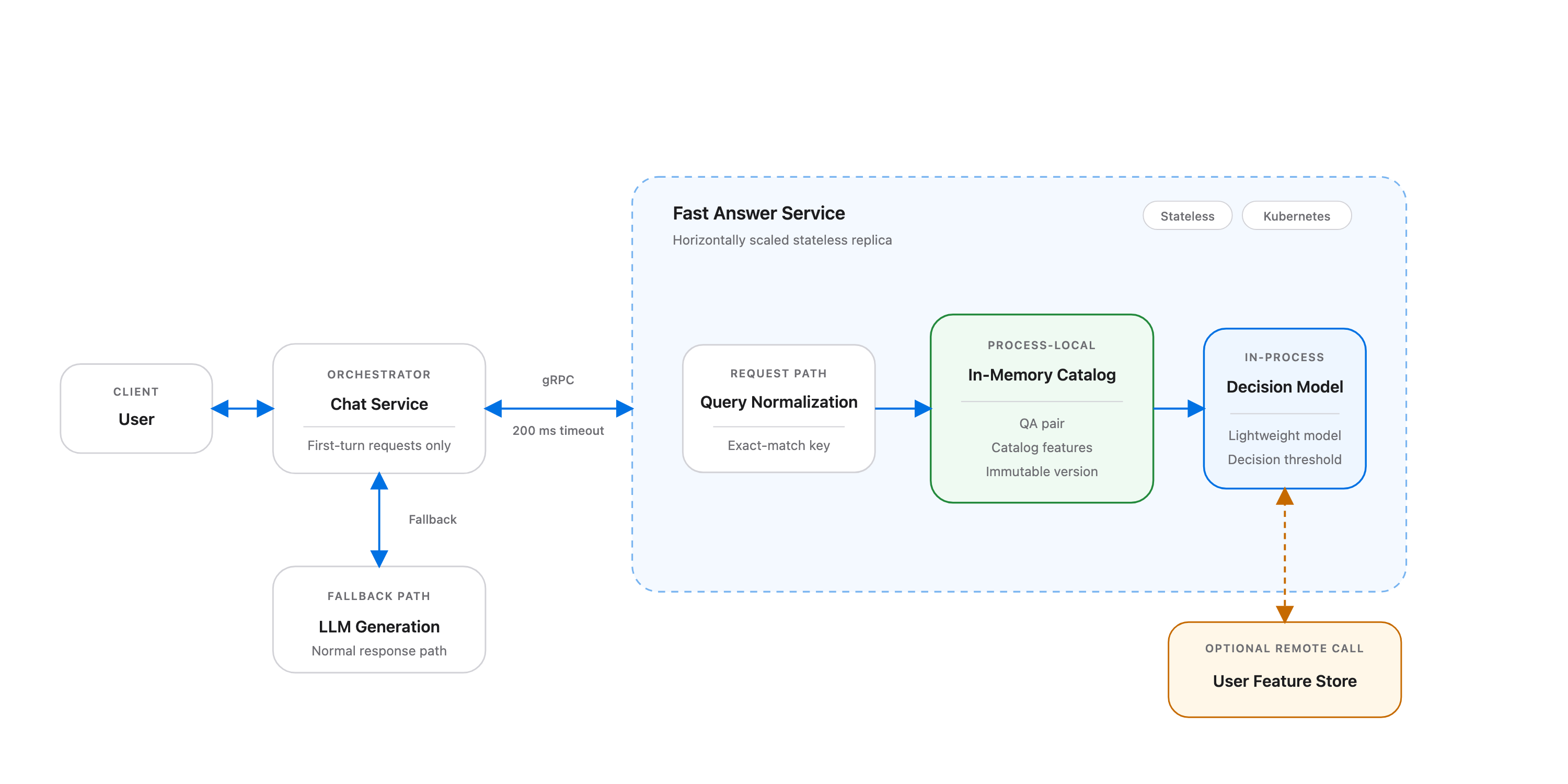
Figure 1. Online serving architecture of the Fast Answer system.
The Fast Answer Service itself should be stateless and deployed as a horizontally scalable service on Kubernetes. The Chat Service communicates with it through gRPC.
A stateless design allows the service to scale horizontally as traffic changes. Requests can be routed to any healthy replica without requiring session affinity, which simplifies load balancing and failure recovery.
Kubernetes is not the only deployment option. A serverless platform could provide automatic scaling with less operational overhead, while a fixed pool of virtual machines would be simpler to operate at small scale. However, the workload assumed here has both high sustained traffic and a strict p99 latency requirement. Maintaining a pool of warm replicas provides more predictable tail latency than relying on serverless instances that may experience cold starts.
I would therefore accept the additional operational complexity of Kubernetes in exchange for predictable warm capacity, horizontal scaling, rolling deployments, and controlled traffic rollout.
For communication between the Chat Service and Fast Answer Service, I would use gRPC rather than a JSON-based REST API. This is an internal, high-QPS service-to-service call where compact serialization and strongly typed interfaces are useful. The trade-off is additional schema management through Protocol Buffers and somewhat less convenient manual debugging compared with HTTP/JSON.
3.2 Retrieval Store: An Immutable In-Memory Catalog
The first version of Retrieval uses exact query matching. This makes the serving requirement substantially simpler than that of a general-purpose search system:
\[\text{Normalized Query} \rightarrow \text{Catalog Entry}.\]A conventional design might place the Catalog behind Redis or another distributed key-value store. Redis would provide low-latency lookups, replication, and independent updates to the serving data. However, every lookup would still introduce an additional network hop and another dependency on the critical path.
Instead, I would first investigate whether the entire serving Catalog can be loaded directly into the memory of each Fast Answer Service replica.
Each Catalog version would be published as an immutable artifact. When a Fast Answer Service replica starts, it downloads the selected Catalog version and loads a mapping from normalized query to QA entry into memory. Retrieval then becomes a local hash-table lookup.
Normalized Query
        ↓
In-Memory Hash Lookup
        ↓
QA Pair + Catalog Features
This design has several advantages for the current workload:
- No network call is required for retrieval.
- Exact-match lookup is extremely cheap.
- Retrieval availability is coupled only to the health of the serving process itself.
- Every request is served against a known Catalog version.
The main question is whether the Catalog is small enough to replicate in memory across all serving pods. The assumptions from Section 2 allow a rough upper-bound estimate.
The assumed human-review capacity is approximately 7,200 query candidates per day. Even if the initial Catalog construction runs for 30 days and every reviewed query is approved, the Catalog would contain at most:
\[N_{\text{Catalog}} \leq 7{,}200 \times 30 = 216{,}000\]entries.
The actual number would likely be smaller because some queries would fail eligibility review and some generated answers would fail answer review. For capacity planning, a Catalog of approximately 200K entries is therefore a conservative initial estimate.
Suppose each entry contains approximately:
- 100 bytes for the normalized query
- 2 KB for the prepared Fast Answer
- 500 bytes for Catalog metadata and precomputed Decision features
The serialized data is therefore roughly 2.6 KB per entry. Allowing approximately 2× overhead for strings, hash-table structures, and the in-memory representation gives a conservative estimate of roughly 5 KB per entry.
The resulting memory footprint is:
\[200{,}000 \times 5\text{ KB} \approx 1\text{ GB}.\]A roughly 1 GB Catalog can comfortably fit in the memory of each Fast Answer Service replica. Even allowing additional memory for the service process and Decision model, an instance with several gigabytes of memory should be sufficient.
Even if the human-review bottleneck were reduced and Catalog construction throughput improved by 10×, the same estimate would produce a Catalog of roughly 2 million entries, or about 10 GB per replica. That is still practical for a memory-optimized serving instance, so process-local replication would remain a reasonable choice at that scale.
3.3 Feature Serving
The Decision model uses two broad categories of features: Catalog-entry features and user features.
Catalog-entry features, such as historical uplift, answer age, feedback volume, and query frequency, are naturally associated with the retrieved QA entry. These features should therefore be packaged directly with the Catalog artifact.
A successful retrieval would return both the answer and its precomputed features:
Catalog Entry
  ├── Query
  ├── Answer
  ├── Historical Uplift
  ├── Query Frequency
  ├── Catalog Age
  └── Other Precomputed Features
This avoids a separate feature-store lookup for data that changes relatively slowly and can be recomputed during Catalog publication.
User-level features are different. Features such as historical Fast Answer affinity or recent regeneration behavior may need to be fetched from an online feature store.
Adding this remote call, however, directly consumes part of the 200 ms p99 latency budget and introduces another dependency on the serving path.
I would therefore make the inclusion of user features conditional on their demonstrated predictive value.
The initial Decision model would first be evaluated using only features already available in the request and Catalog entry. I would add a remote user-feature lookup only if offline and online experiments show that the additional features produce a meaningful increase in Fast Answer serve rate under the same satisfaction constraint.
3.4 Decision Model Serving
The first learned Decision model described in Part 1 does not require a large neural network. A logistic regression model, GBDT, or similarly lightweight model should be sufficient as an initial implementation.
For a model of this size, I would not deploy a separate model-serving system such as Triton or a dedicated inference microservice. Instead, the model would be loaded directly into the Fast Answer Service process and evaluated in-process.
Retrieved QA + Features
        ↓
In-Process Decision Model
        ↓
Estimated Satisfaction Impact
        ↓
Decision Threshold
        ↓
Serve / Fall Back
This removes another network hop from the critical path and allows Decision inference to remain extremely cheap.
The trade-off is tighter coupling between the Decision model and the Fast Answer Service. Updating the model requires updating the artifact loaded by the service, and the model cannot scale independently from the rest of the Fast Answer Service.
For the current system, I would accept that trade-off. The model is small, and the Catalog itself already requires periodic version updates. Catalog and Decision model versions can therefore be packaged as part of the same serving release.
A serving bundle might look like:
Fast Answer Release v42
  ├── Catalog v42
  ├── Catalog Features v42
  ├── Decision Model v17
  └── Decision Threshold v8
New pods can start with the new bundle while existing pods continue serving the previous version.
This also allows gradual rollout. Kubernetes can run both old and new replica sets simultaneously and shift traffic incrementally. If metrics regress, traffic can be shifted back to the previous version without rebuilding the Catalog or model.
3.5 Additional Considerations
Fast Answer Service replicas should be deployed in the same regions as the Chat Service, with the same immutable serving bundle replicated across regions. This avoids adding a cross-region network hop to the latency-critical path.
Special care is also required to keep query-normalization logic consistent between the online and offline paths. A Catalog key produced by the offline pipeline must be identical to the key produced from the same query during online serving; otherwise, valid entries will become false misses.
The system also requires proper observability across the Chat Service, Fast Answer Service, Catalog, Decision model, and fallback path. I will discuss the monitoring and operational details in Part 3.
4. Offline Architecture
The offline architecture has two responsibilities: constructing the QA Catalog and training the Decision model. The Catalog pipeline consumes historical chat logs to discover new QA opportunities and production feedback to identify existing entries that should be updated or deleted. Both offline pipelines process large-scale logs, but their final outputs are small enough to be packaged directly into the immutable serving bundle described in Section 3.

Figure 2. Offline architecture of the Fast Answer system.
4.1 Log Storage and Incremental Aggregation
Historical chat logs and production feedback are stored in object storage in a columnar format such as Parquet. Production feedback includes the served Catalog entry, entry-level traffic, thumbs-down feedback, and regeneration or retry behavior. Given the estimated scale of 25 billion queries for the initial 30-day backfill, Spark is a reasonable choice for distributed filtering, normalization, and aggregation.
The initial backfill should process these logs as daily partitions. This makes incremental updates to a 30-day sliding window straightforward: remove the oldest daily partition, add the newest one, and recompute the aggregate over the remaining 30 days. Each partition is processed independently, so the window can be refreshed without rescanning the complete raw history.
The pipeline produces two derived datasets. Normalized query counts feed the path that discovers new Catalog entries, while entry-level feedback aggregates feed the path that proposes updates and deletions. This avoids rescanning approximately 25 billion raw records whenever the Catalog is rebuilt. The expensive raw-log processing happens only once per daily partition, while subsequent Catalog builds operate on much smaller aggregated representations.
I prefer this approach over maintaining a single continuously updated global frequency table. Daily aggregates can remain immutable, which makes backfills and recovery simpler. If processing for one day is incorrect, that partition can be recomputed independently and the 30-day aggregate rebuilt from the corrected result.
This composition works naturally for additive statistics such as query counts and feedback counts. More complex statistics may require additional mergeable state. Query frequency is the primary signal for discovering new Catalog entries, while production feedback provides the primary signals for updating or deleting existing entries.
4.2 Candidate Generation and Human Review
Both offline paths produce candidates for human review. As estimated in Section 2, the assumed review capacity is approximately 7,200 candidates per day, so each path must reduce its aggregated data to a small set of high-value candidates.
Add Candidates
The 30-day query aggregation still produces far more queries than humans can review. The initial system can keep candidate generation simple: queries already covered by the Catalog are removed, basic eligibility rules filter obvious non-candidates, and the remaining queries are ranked primarily by traffic frequency.
30-Day Query Frequency
        ↓
Remove Existing Catalog Entries
        ↓
Eligibility Rules
        ↓
Rank by Expected Coverage Gain
        ↓
Top Candidates within Review Budget
Update and Delete Candidates
The second path aggregates production feedback for existing Catalog entries. Entries with unusually negative feedback, increasing regeneration or retry behavior, or freshness concerns become update candidates. Entries with persistently low traffic or severe quality problems can become delete candidates.
These rules do not mutate the Catalog directly. They produce a prioritized set of update and delete candidates that joins the add candidates at the human-review stage.
At this point, the problem is no longer a distributed-compute bottleneck. Spark may process hundreds of millions of records upstream, but the combined output of both paths should be only thousands of review candidates per day.
The selected candidates can then be written to PostgreSQL, which serves as the backend for the internal review workflow. A relational database is appropriate here because the workload is relatively small and the important requirements are transactional state transitions and auditability rather than large-scale analytical processing.
The review workflow depends on the proposed action:
PENDING_REVIEW
  ├── ADD_APPROVED → ANSWER_GENERATING → ANSWER_REVIEW
  ├── UPDATE_APPROVED → ANSWER_GENERATING → ANSWER_REVIEW
  └── DELETE_APPROVED → DELETED
PostgreSQL also becomes the source of truth for the Catalog management workflow. The online serving system does not query this database directly.
4.3 Catalog Mutation and Answer Generation
Approved add candidates proceed to answer generation. Update candidates may also require a newly generated answer, while approved delete candidates can be removed without generation. Because the upstream filtering stage reduces hundreds of millions of daily records to at most thousands of reviewed candidates, answer generation does not require a large dedicated serving system.
A durable task queue and a small pool of stateless generation workers should be sufficient. Each job contains the approved query or existing Catalog entry together with its generation configuration, and the result is written back to PostgreSQL for final human review.
The queue provides retry and failure isolation without coupling answer generation to the review application. Generation throughput can also be scaled independently if review capacity increases.
Once an answer for an add or update candidate passes review, the approved QA pair is written to the Catalog source of truth. An approved deletion marks the entry for exclusion from the next Catalog snapshot. The Catalog table would contain the information required to construct the serving artifact, including:
Catalog Entry
  ├── Normalized Query
  ├── Fast Answer
  ├── Query Frequency
  ├── Historical Feedback
  ├── Catalog Age
  ├── Human Review Metadata
  └── Precomputed Decision Features
The Catalog itself remains mutable in PostgreSQL as entries are added, updated, or removed. Online serving, however, consumes only immutable snapshots built from an approved Catalog state.
4.4 Decision Model Training Pipeline
The Decision model is trained from the randomized experiment data described in Part 1. The raw experiment logs are stored in the same object-storage-based data platform used by the Catalog pipeline.
The scale requirements of data preparation and model training are different. Experiment logs may contain hundreds of millions of requests, so feature generation and training-dataset construction should use Spark. The actual Decision model, however, is expected to be a logistic regression, GBDT, or similarly lightweight model.
Distributed computation should handle data preparation, while the model itself can be trained on a single CPU machine using a library such as scikit-learn or XGBoost. There is little benefit in introducing distributed model-training infrastructure for a model this small.
After training, candidate thresholds are evaluated on randomized holdout data using the off-policy evaluation procedure described in Part 1:
\[t^* = \arg\max_t \operatorname{ServeRate}(t) \quad \text{s.t.} \quad \widehat{\Delta S}_{\text{OPE}}(t) \ge -\epsilon.\]The output of the training pipeline is therefore not only a model artifact but also the selected Decision threshold.
Decision Model v17
Decision Threshold v8
Both are versioned independently so that a threshold can be changed without necessarily retraining the model.
4.5 Building and Publishing the Serving Bundle
The Catalog and Decision pipelines eventually converge into a single release artifact.
Approved Catalog
      ↓
Catalog Snapshot
      │
      ├──────────────┐
      │              │
Decision Model       │
Decision Threshold   │
      │              │
      └──────┬───────┘
             ↓
      Release Build
             ↓
Fast Answer Release v42
  ├── Catalog v42
  ├── Catalog Features v42
  ├── Decision Model v17
  ├── Decision Threshold v8
  └── Normalization Version v7
             ↓
Versioned Object Storage
             ↓
Kubernetes Rollout
The normalization version is included because offline Catalog construction and online Retrieval must produce exactly the same Catalog key for the same query. A normalization change must therefore be deployed together with a compatible Catalog snapshot.
The release artifact is immutable and stored in versioned object storage. When a new Fast Answer Service pod starts, it downloads the configured release, validates the artifact, loads the Catalog and Decision model into memory, and becomes ready to receive traffic only after initialization succeeds.
This allows old and new releases to coexist during a rollout. If the new release causes a regression, traffic can be moved back to pods running the previous immutable bundle.
This design deliberately moves complexity away from the online critical path. Catalog management, large-scale aggregation, model training, validation, and artifact construction all happen offline. The resulting online system only needs to load a verified bundle and execute local retrieval and lightweight Decision inference.
5. Failure Handling and Capacity Validation
The Fast Answer path must remain optional from the Chat Service’s perspective. Each request receives a 200 ms hard timeout. A Fast Answer Service miss, error, or timeout causes the Chat Service to fall back to normal LLM generation, so a Fast Answer failure cannot disrupt the existing response path.
A circuit breaker provides protection against persistent failures. If the Fast Answer Service remains unhealthy, the Chat Service should temporarily stop calling it and route requests directly to LLM generation. On the serving side, a new pod should pass readiness checks only after it has downloaded, loaded, and validated its Catalog and Decision model artifacts.
Capacity should be determined through load testing rather than by guessing a replica count. The sustainable QPS of one fully initialized pod should be measured under a realistic request mix and verified against the 200 ms p99 latency budget. The required replica count can then be calculated as:
\[N_{\text{replicas}} = \left\lceil \frac{\text{QPS}_{\text{peak}}}{\text{QPS}_{\text{per replica}}} \times \text{Headroom Factor} \right\rceil.\]The final load test should verify the approximately 30K QPS peak target from Section 2 with enough headroom for traffic spikes, pod failures, and rolling deployments.
6. Wrap-up
This post was intended as an architectural overview rather than a complete production design document. My goal was to identify the major infrastructure decisions that are specific to this system and reason about them from the scale and latency assumptions established earlier.
As a result, I intentionally left out general-purpose infrastructure concerns such as authentication, network configuration, access control, and other platform-level details that would be required in a real production system but are not particularly specific to Fast Answers.
There are also important questions around observability, deployment, experimentation, and ongoing operations that I have only briefly touched on here. These become especially important once the system is running in production and the Catalog, Decision model, and user traffic continuously change.
I will cover those topics in Part 3, focusing on how I would monitor, operate, and continuously improve the system after launch.
If you have read this far, something in this post probably caught your interest. If you would like to know more about me, feel free to connect with me on LinkedIn.