TL;DR

• Part 1 turns the product observations from Part 0 into a business objective and an ML system design.
• This post is less about sophisticated model architectures and more about how to translate a business objective into concrete ML problems.

This is a four-part series:
Part 0. Product Teardown and Related Work
Part 2. Production Architecture
Part 3. Operations and Continuous Improvement

1. Business Context & Objective

1.1 Business Objective

Part 0 examined Fast answers from the outside: observable product behavior, related products, and relevant research. From this point on, I will imagine the reasoning that might have justified this project when OpenAI first began considering it internally. This may differ substantially from OpenAI’s actual thought process, but I wrote it for the fun of designing one product end to end.

A reasonable business objective for introducing Fast answers would be:

Reduce inference cost and latency without degrading user satisfaction.

This section briefly justifies that objective, then defines the domain assumptions and metrics used throughout the rest of the design.

1.2 Traffic Scale and Cacheable Opportunity

OpenAI’s internal data analysts and scientists were probably already studying the wide range of user queries. They would be able to estimate how often recurring information-seeking queries appear each day, what share of them are duplicates, and how many could be answered with a cached response. A question such as Why is the sky blue? has a stable answer over time, so a cached response may be sufficient.

ChatGPT operates at enormous scale. OpenAI’s report How People Use ChatGPT states that the product received 2.5 billion messages per day in 2025, with 24% classified as Seeking Information.¹ This design applies Fast Answers only to the first query in a new chat, so the exact addressable traffic is unknown, but the scale is still informative.

The next question is how much of that traffic is repetitive and cacheable. Query frequencies in web search are often highly skewed, suggesting that a relatively small set of frequent queries may account for a meaningful share of traffic. ChatGPT may follow a different distribution, so applying a specific rule such as 80/20 would be questionable. Still, even 1% of the 600 million daily information-seeking messages would correspond to 6 million requests per day.

This motivates the working assumption that a relatively small prepared-answer catalog could cover a non-trivial share of eligible first-turn queries. Each successful cache hit replaces an otherwise necessary LLM generation, creating meaningful opportunities to reduce both inference cost and latency.

1.3 Estimating Potential Savings

A simple general expression for the resulting savings is:

\[\begin{aligned} \text{Daily Savings} &= N_{\text{new chats}} \times P_{\text{info}} \times P_{\text{eligible}\mid\text{info}} \\ &\quad \times \text{HitRate} \\ &\quad \times \left(C_{\text{generation}} - C_{\text{fast}}\right) \end{aligned}\]

• $N_{\text{new chats}}$ is the unknown number of new conversations per day.
• $P_{\text{info}}$ is the unknown probability that the first query is information-seeking.
• $P_{\text{eligible}\mid\text{info}}$ is the unknown probability that an information-seeking first query is eligible for a Fast answer.
• $\text{HitRate}$ is determined by the system discussed in this series.
• $C_{\text{generation}}$ is the unknown internal generation cost.
• $C_{\text{fast}}$ is the much smaller lookup and serving cost.

This expression does not include the increase in user satisfaction from lower latency or the additional value created by freeing GPU capacity.

1.4 Domain Assumptions

• A meaningful portion of traffic is information-seeking and cacheable.
• Fast answers are applied only to the first query in a new chat, since a subsequent query implicitly demands context from the prior conversation.
• Returning a cached answer is always cheaper than generating a new answer.
• Some users may not be satisfied with a cached answer.
• The initial system supports English queries only.

The decisions in the rest of this design will be based on these assumptions.

1.5 Metrics

Primary metrics

• Inference cost reduction
• Latency reduction

Guardrail metrics

• User satisfaction, measured through negative feedback such as thumbs-down
• Regeneration or retry rate²

2. Problem Formulation & ML Objective

2.1 From the Business Objective to Fast Answer Serve Volume

The business objective can be written as:

\[\begin{aligned} \max_{\pi}\quad &\text{Cost Saving}_{\pi} + \alpha\,\text{Latency Saving}_{\pi} \\ \text{subject to}\quad &\text{Satisfaction}_{\pi} \geq \text{Satisfaction}_{\text{LLM}} - \epsilon \end{aligned}\]

This objective means that the Fast Answer system $\pi$ should maximize cost and latency savings while ensuring that user satisfaction is not lower than when users receive LLM-generated answers. The $\epsilon$ term accounts for noise in the observed satisfaction metric.

As assumed above:

\[\text{Cost}_{\text{Fast}} \ll \text{Cost}_{\text{LLM}}, \qquad \text{Latency}_{\text{Fast}} \ll \text{Latency}_{\text{LLM}}\]

Based on the domain assumptions above, serving an answer through the Fast Answer path always saves generation cost and latency. The cost and latency savings from each Fast Answer are therefore always positive. Let the combined saving per served Fast Answer be approximated as a constant $K > 0$. Then:

\[\text{Total Saving} \approx K \times N_{\text{Fast Answer Served}}\]

Total saving is therefore approximately proportional to the number of Fast Answers served. The business objective can be approximated as:

\[\begin{aligned} \max\quad &N_{\text{Fast Answer Served}} \\ \text{subject to}\quad &\text{User Satisfaction} \geq \text{Baseline} - \epsilon \end{aligned}\]

In plain language:

Serve as many requests as possible with Fast Answers without degrading user satisfaction.

If cached answers could satisfy users unconditionally, always serving a Fast Answer would preserve satisfaction and maximize savings. In reality, Fast Answers cannot be served for every request:

• Catalog failure: no satisfactory, fresh, reusable answer exists.
• Retrieval failure: such an answer exists, but the system does not retrieve it.
• Decision fallback: the right answer is retrieved, but the policy falls back to LLM generation.

The objective therefore remains maximizing the number of Fast Answers served subject to the satisfaction constraint. The serving volume is determined by how many opportunities the Catalog creates, how many Retrieval finds, and how many the Decision Policy converts into Fast Answers. Satisfaction remains a separate aggregate constraint on the overall serving policy.

2.2 Decomposing Fast Answer Serve Volume

The next step is to decompose how the Fast Answer serve volume is produced. Ideally, the objective would be optimized end to end. However, dividing the problem into subproblems based on the funnel and failure cases implied by the domain knowledge above makes it much easier to solve. Although not optimizing the objective directly may introduce some loss, each individual problem can be solved more easily and accurately, potentially producing better overall performance. This type of staged approach is common in search and recommendation systems.

At least three events must occur in sequence:

\[\begin{aligned} A &= \{\text{A satisfactory reusable answer exists in the catalog}\} \\ R &= \{\text{The correct catalog answer is retrieved}\} \\ D &= \{\text{The decision policy serves the retrieved answer}\} \end{aligned}\]

Under this sequential decomposition, the expected Fast Answer serve volume can be expressed as:

\[\mathbb{E}\left[N_{\text{Fast Answer Served}}\right] = N_{\text{Total Traffic}} \times \underbrace{P(A)}_{\text{Catalog Coverage}} \times \underbrace{P(R \mid A)}_{\text{Retrieval Quality}} \times \underbrace{P(D \mid A,R)}_{\text{Decision Serve Rate}}\]

From this decomposition, each of the three modules (Catalog, Retrieval, and Decision Policy) should have its own objective and metrics.

2.3 Module-Level Objectives and Metrics

Module 1 — Catalog Construction

Question

Do we have a satisfactory reusable answer for this query?

Input → Output

Historical query traffic → Prepared QA catalog

Objective

Maximize catalog coverage: the fraction of eligible traffic for which a satisfactory reusable answer exists.

\[\max P(A)\]

Metrics

• Primary: Traffic-weighted Coverage
• Guardrails: Answer Quality, Freshness, Safety

Module 2 — Retrieval

Question

If a reusable answer exists, can we find the right one?

Input → Output

User query + QA catalog → Best candidate QA pair

Objective

\[\max P(R \mid A)\]

Maximize the retrieval success rate, given that an appropriate answer exists.

Metrics

• Primary: Top-1 Compatibility or Precision@1
• Secondary: Recall@K, False-match Rate

Module 3 — Decision Policy

Question

If we found the right answer, should we actually serve it?

Input → Output

User query + retrieved QA + available context → Serve Fast Answer / Fall back to LLM

Objective

The Decision Policy should maximize the Fast Answer serve rate while maintaining the satisfaction guardrail:

\[\begin{aligned} \max\quad &\text{Fast Answer Serve Rate} \\ \text{subject to}\quad &\Delta S \geq -\epsilon \end{aligned}\]

Here, $\Delta S$ represents the change in user satisfaction under the Fast Answer policy relative to always using LLM generation.

This may look similar to the global business objective, but it operates only after the upstream Catalog and Retrieval stages have succeeded. Under the earlier assumption that each Fast Answer produces approximately the same cost and latency saving, the remaining Decision problem reduces to identifying the requests for which that saving can be realized with an acceptable impact on user satisfaction.

This objective can be further reduced to a prediction problem. Let $x$ represent the information available to the Decision Policy, such as the user query, retrieved answer, and available user or contextual features. Let

\[\pi(x) \in \{0,1\}\]

denote the policy, where $\pi(x)=1$ means serving the Fast Answer and $\pi(x)=0$ means falling back to LLM generation.

For each request, define the expected satisfaction impact of serving the Fast Answer instead of the LLM as

\[\tau(x) = \mathbb{E}\left[ S_{\text{Fast}}-S_{\text{LLM}} \mid X=x \right].\]

The main modeling challenge is that $\tau(x)$ is not directly observable for an individual request, since the same request cannot simultaneously receive both a Fast Answer and an LLM response. Section 6 discusses how randomized experimental data can be used to estimate it.

The Fast Answer serve rate is then

\[\mathbb{E}[\pi(X)].\]

Because requests with $\pi(X)=0$ still receive the baseline LLM response, the aggregate satisfaction change introduced by the policy is

\[\mathbb{E}[\pi(X)\tau(X)].\]

Therefore, the Decision Policy objective becomes

\[\begin{aligned} \max_{\pi}\quad &\mathbb{E}[\pi(X)] \\ \text{subject to}\quad &\mathbb{E}[\pi(X)\tau(X)] \geq -\epsilon. \end{aligned}\]

Using Lagrangian relaxation, this can be written as

\[\mathcal{L}(\pi,\lambda) = \mathbb{E}[\pi(X)] +\lambda\left(\mathbb{E}[\pi(X)\tau(X)]+\epsilon\right), \qquad \lambda \geq 0.\]

Rearranging,

\[\mathcal{L}(\pi,\lambda) = \mathbb{E}\left[\pi(X)(1+\lambda\tau(X))\right] +\lambda\epsilon.\]

For a fixed $\lambda$, the optimal policy is therefore

\[\pi(x) = \begin{cases} 1, & \text{if } 1+\lambda\tau(x)>0, \\ 0, & \text{if } 1+\lambda\tau(x)<0. \end{cases}\]

The original constrained optimization problem can therefore be implemented by estimating $\tau(x)$, the expected satisfaction impact of serving a Fast Answer instead of an LLM response, and choosing a threshold that maximizes the serve rate while satisfying the aggregate satisfaction constraint.

The Lagrange multiplier $\lambda$ controls the trade-off between serving more Fast Answers and preserving satisfaction. In practice, rather than explicitly optimizing $\lambda$, I would sweep the decision threshold on held-out experimental data and choose the lowest threshold whose estimated satisfaction delta still satisfies the guardrail. This yields the highest Fast Answer serve rate among policies that meet the satisfaction constraint.

Metrics

• Primary: Fast Answer Serve Rate
• Guardrail: Satisfaction Delta

2.4 Connecting Module Objectives to Business Value

The complete relationship can be summarized with one equation:

\[\begin{aligned} \mathbb{E}\left[N_{\text{Fast Answer Served}}\right] = N &\times \underbrace{P(A)}_{\text{Catalog Coverage}} \\ &\times \underbrace{P(R \mid A)}_{\text{Retrieval Success}} \\ &\times \underbrace{P(D \mid A,R)}_{\text{Decision Serve Rate}} \end{aligned}\]

and:

\[\mathbb{E}[\text{Business Saving}] \approx K \times \mathbb{E}\left[N_{\text{Fast Answer Served}}\right]\]

The logic is therefore:

\[\begin{gathered} \uparrow\text{Catalog Coverage},\quad \uparrow\text{Retrieval Quality},\quad \uparrow\text{Decision Serve Rate} \\ \Downarrow \\ \uparrow\text{Fast Answer Serve Volume} \\ \Downarrow \\ \uparrow\text{Cost and Latency Saving} \\ \text{subject to Satisfaction Delta} \geq -\epsilon \end{gathered}\]

This explains why optimizing each module’s local objective should improve the global business objective.

The reason to define this framework before designing the individual modules is that it provides debuggability and prioritization. If the complete system underperforms, module-level objectives and metrics make it possible to isolate the root cause and decide where further investment will have the greatest impact.

Additionally, each module does not need to be a fancy deep-learning model. For each module, define what goes in, what comes out, what should be optimized, and how success is measured.

3. High-Level Architecture

3.1 High-Level Architecture

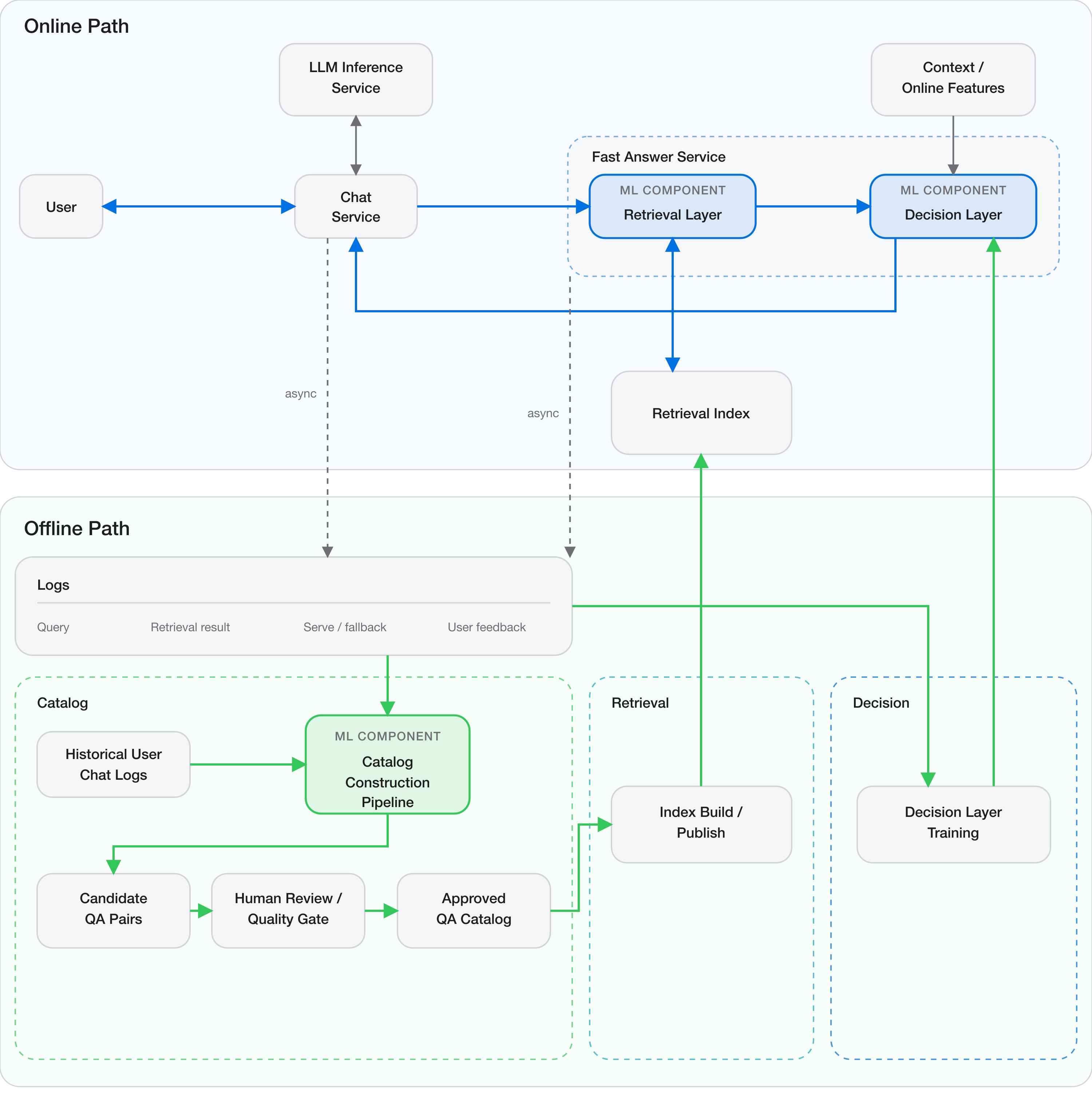
Figure 1. High-level architecture of the Fast Answer system.

The high-level architecture is divided into two paths. The first is the online path that handles user requests. When a request reaches the Chat Service, it calls the Fast Answer Service first for the initial query in a chat. If the Fast Answer Service returns an answer, the Chat Service immediately sends it back to the user. Otherwise, it invokes LLM generation.

Within the Fast Answer Service, the Retrieval Layer first searches a prebuilt index for a candidate QA pair. The Decision Layer then determines whether that candidate should be shown. It combines the candidate QA pair with context from the online feature store to make the final decision. Each stage must also log its outputs asynchronously so that the data can later support analysis and model training.

The offline path uses accumulated logs to build the QA catalog. An automated pipeline extracts candidate QA pairs, which pass through a review process before entering the final catalog. This process may add new QA pairs or update and remove existing ones. A periodic job then builds the retrieval index from the catalog. The Decision Layer should also be continuously retrained on newly collected data and updated when a new model is ready.

A more complete system would require additional discussion of retrieval-model training, feature-store pipelines, deployment, A/B testing, and other production concerns. The diagram shows only the components most central to the ML design. The technical implementation and operational details will be covered in later posts.

3.2 Heuristic-Based V0

Suppose the first Fast Answer system is implemented and launched from this architecture. Because the Catalog, Retrieval, and Decision layers are modularized, the work can be divided across the available team. If I had to build it alone, however, the first version would exclude complex ML components and focus on getting the complete system running. Section 2 defines each module’s objective as an ML problem, but the launch version does not necessarily need an ML model.

For example, the Catalog module could use exact matching to find high-frequency queries, generate LLM answers for them, and send those answers through manual review. Retrieval could use an index built for exact matching. After upstream eligibility checks pass, an experiment assignment layer could randomly assign a small fraction of traffic to either a Fast Answer or LLM generation. None of these approaches is sophisticated, but together they provide a set of heuristics that should behave reasonably well for an initial launch.

3.3 What Should We Improve Next?

Suppose the system is now running with heuristic-based modules. The next step is to experiment on a small fraction of traffic, verify that the system and business metrics are healthy, and confirm that the required logs are being collected correctly. Once those checks pass, each module can be improved against the objectives defined earlier.

If resources allow only one module to be improved first, I would choose the Decision Layer. The Catalog should already work reasonably well because every entry passes through manual review, even though that review is expensive. Exact-match Retrieval is deliberately high precision. The largest uncertainty immediately after launch is therefore: Should this retrieved answer actually be shown? This decision sits closest to the satisfaction guardrail. Because the V0 experiment assignment is randomized at the chat-session level, it also provides controlled comparison data for learning a policy.

Using this randomized data to train a learned Decision Layer would make it possible to incorporate user context and make better serving decisions. For example, the system could show more Fast Answers to users who are usually satisfied with them.

The Catalog would be my second priority. Automating part of the manual-review process is likely to have high ROI. It would reduce review costs, and the work required for automation would force the team to define the intended behavior of Fast Answers more precisely. The knowledge and data accumulated during V0 operation would make that definition easier.

Retrieval would come last. Once the Catalog work has clarified the product objective, the system could begin moving from exact matching toward semantic matching. This ordering follows from the example in Part 0, where a general-purpose text embedder was not aligned with answer equivalence.

The remainder of this post focuses on the modeling design for the three components, with particular emphasis on the Decision Policy as the first learned optimization target. Even when the Catalog or Retrieval modules remain heuristic-based, the discussion will cover what data should be used to evaluate and launch them. It will also briefly introduce possible approaches for more advanced modeling.

4. Catalog

The Catalog system is essentially a system that extracts information satisfying a particular set of conditions from chat logs offline and stores only a selected subset. Those conditions may require a query to occur frequently, ask for information, support a stable answer, and satisfy other product requirements.

This is a well-known industry pattern. Structurally, this resembles offline indexing and knowledge-base construction systems: extract information useful for a specific serving objective, filter it, and publish it in a retrievable form. Examples include search indexing and ChatGPT’s recently introduced improved Memory feature.³

4.1 Catalog Lifecycle

As discussed above, I would begin with a heuristic-based system. The full lifecycle would look like this:

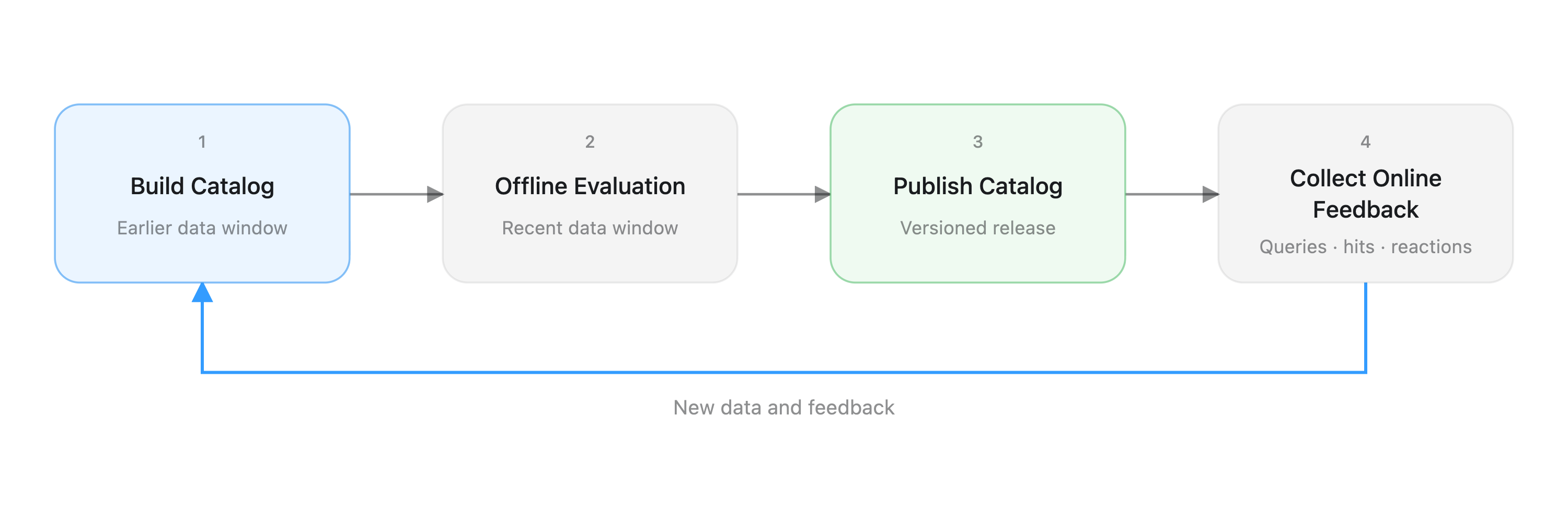
Figure 2. Build the catalog, evaluate it on recent data, publish it, collect online feedback, and repeat.

The sequence is straightforward. Build the catalog from a slightly older data window, evaluate it offline on recent data, publish it, collect feedback from production, and rebuild it with new data. The iteration cadence depends on how frequently the query distribution changes. It would be better to iterate more frequently at the beginning. Once the catalog has converged to some degree, a longer iteration cycle should be acceptable.

4.2 Heuristic-Based Catalog Build

Catalog construction has three paths: adding new QA pairs, deleting existing QA pairs, and updating existing answers.

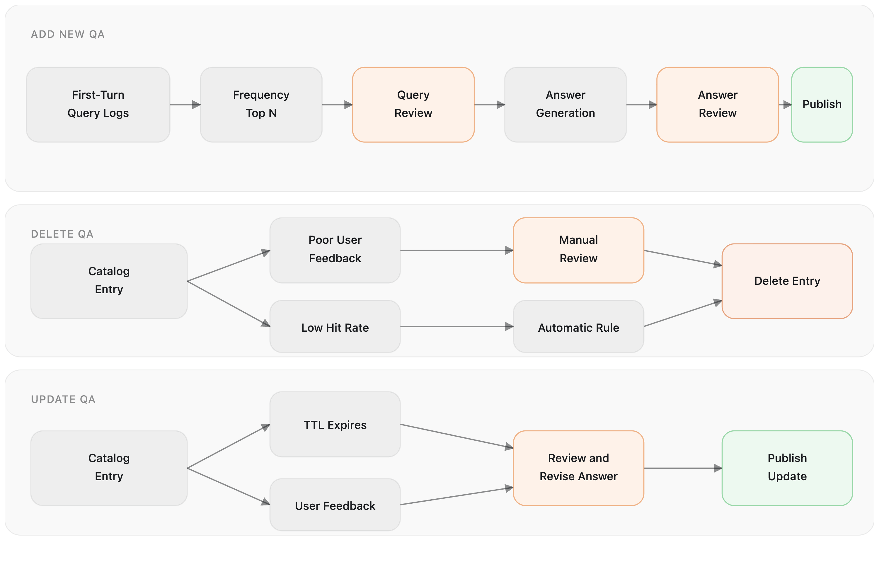
Figure 3. The three paths in the heuristic-based catalog construction system.

Adding New QA Pairs

The first path adds a new QA pair through three stages:

1. Query extraction and manual review
2. Answer generation and manual review
3. Catalog publishing

Query extraction begins by pulling a list of first-turn queries from chat logs. The system counts them using exact matching and selects the top $N$ most frequent queries. A human then filters this list for information-seeking queries.

Next, a separate LLM generates an answer for each approved query. Reusing an answer from existing chat logs would be risky for two reasons. First, the answer may contain personalized information because the model may have used memory. Second, a Fast Answer may require its own target length and tone.

Generating a fresh answer is therefore a reasonable choice. The generated answer also passes through manual review. An approved QA pair is then published to the catalog.

Deleting QA Pairs

The second path removes QA pairs. Many heuristic rules are possible, but two signals are especially important:

• Poor user feedback
• Low hit rate

An entry with consistently poor user feedback can be sent through manual review and deleted. An entry with sufficiently low traffic can be removed automatically when catalog maintenance or review cost matters.

Updating QA Pairs

The third path updates QA pairs. The clearest reason to update an entry is that its answer has become outdated, but automatically detecting this is difficult. A simple solution is to assign a TTL to each answer and review it when the TTL expires. User feedback can also trigger manual review and an answer update.

Updating a question does not need a separate path. In practice, changing a question is equivalent to deleting the old entry and adding a new one.

The design above assumes that every manual review is performed by a person. An LLM Judge could make this process faster, but simply prompting an LLM would not be sufficient. The process described in LLM-as-a-Judge in Practice provides a better way to build one, so I will not repeat that discussion here.

4.3 Offline Evaluation

Even a heuristic-based catalog requires evaluation before deployment. As discussed in Section 2, the Catalog’s role is to maximize coverage of QA pairs eligible for Fast Answers. The evaluation split should therefore be time-based: build the catalog from historical data, then measure traffic-weighted catalog coverage on more recent data.

The metric can be written as:

\[\text{Traffic-Weighted Coverage} = \frac{ \sum_{q \in Q_{\mathrm{recent}}} n_q \cdot \mathbb{1}[q \text{ has a satisfactory reusable answer in the catalog}] }{ \sum_{q \in Q_{\mathrm{recent}}} n_q }\]

Here, $n_q$ is the number of times query $q$ appears in the recent evaluation window.

Answer quality, freshness, and safety are the guardrail metrics. The catalog should be independently re-audited on the evaluation date rather than evaluated using the same labels that were used to approve entries. The resulting audit can measure a pass rate for each dimension:

\[\text{Pass Rate}_d = \frac{ \sum_{a \in C} \mathbb{1}[a \text{ passes dimension } d] }{|C|}, \qquad d \in \{\text{quality},\text{freshness},\text{safety}\}\]

The audit labels could use a Likert scale, but I would recommend binary labels. The reason is discussed in LLM-as-a-Judge in Practice.

This produces a heuristic-based catalog system that can still be evaluated with data and deployed with a reasonable degree of confidence.

4.4 Online Evaluation

The online evaluation of the Catalog asks one question:

Is the published catalog creating the opportunities we expected under actual live traffic?

The first metric is Online Catalog Coverage:

\[\text{Online Catalog Coverage} = \frac{ \sum_{q \in Q_{\mathrm{live}}} n_q \cdot \mathbb{1}[q \text{ has an entry in the published catalog}] }{ \sum_{q \in Q_{\mathrm{live}}} n_q }\]

This checks whether the coverage measured offline on a historical window is maintained under actual production traffic.

The second metric is the coverage gain from a newly published catalog:

\[\Delta \text{Coverage} = \text{Coverage}_{\mathrm{new}} - \text{Coverage}_{\mathrm{old}}\]

This measures how much additional traffic the new catalog covers relative to the previous version. It also shows whether newly added QA pairs are actually receiving traffic. If many entries are rarely used, the Catalog Construction process may be inefficient.

Finally, downstream feedback should be aggregated at the catalog-entry level. For every catalog answer that is actually served, useful signals include:

• Thumbs-down feedback
• Regeneration or retry

These signals can trigger the review, update, or deletion paths described above.

4.5 Advanced Directions

A more advanced catalog system should be able to answer the following questions:

• Can query extraction become more robust than simple frequency ranking?
• How can answer generation use user feedback to update answers automatically and improve user satisfaction?
• How far can manual review be reduced? Can the LLM Judge become reliable enough that humans review only hard samples?
• How frequently should the catalog be updated to return stable answers?

5. Retrieval

Retrieval deliberately uses exact matching to keep the system complexity low. When a query arrives, the system looks it up in the catalog. If the exact same query exists, it retrieves the corresponding answer.

From the perspective of query matching, this provides effectively perfect precision. That does not mean the retrieved answer will always satisfy the user. Answer satisfaction still depends on the quality of the QA curation performed by the Catalog system.

Because exact-match Retrieval introduces no additional modeling uncertainty, I would not build a separate ML evaluation pipeline for Retrieval in V0. Basic correctness and index-consistency checks would still be required.

If the system is later extended to retrieve answers for semantically similar queries, see the Retrieval discussion in Part 0.

6. Decision Layer

6.1 Collecting Training Data

The first problem is that the expected satisfaction impact defined in Section 2 cannot be observed directly for an individual request:

\[\tau(x) = \mathbb{E}\left[ S_{\text{Fast}}-S_{\text{LLM}} \mid X=x \right].\]

The same request cannot simultaneously receive both a Fast Answer and an LLM response. V0 should therefore randomize traffic only after it passes the upstream eligibility checks:

Retrieved Valid QA
        ↓
Eligibility Gate
        ↓
Experiment Assignment
   ├── Fast Answer
   └── LLM

For each assigned request, the system should collect:

• $x$: the query, retrieved QA pair, catalog metadata, and available user or contextual features
• Treatment assignment: Fast Answer or LLM
• Satisfaction outcomes, including thumbs-down and regeneration or retry
• A composite satisfaction label, if needed

Randomization makes the two groups comparable and provides the counterfactual evidence needed to estimate the satisfaction impact of Fast Answers.

Even after the Decision Policy is upgraded from V0 to V1, a small fraction of eligible traffic should remain randomized. This continuously provides unbiased data that can be used for future model training and evaluation.

6.2 Estimating Satisfaction Impact

The simplest approach is to fit two outcome models (T-learner). Let $T$ denote the randomized treatment assignment:

\[\widehat{S}_{F}(x) = \mathbb{E}[S \mid T=\text{Fast}, X=x]\] \[\widehat{S}_{L}(x) = \mathbb{E}[S \mid T=\text{LLM}, X=x].\]

The estimated satisfaction impact is then:

\[\widehat{\tau}(x) = \widehat{S}_{F}(x)-\widehat{S}_{L}(x).\]

This is essentially an uplift estimation problem. There is no need to begin with a complex model. Logistic regression, a GBDT, or a small MLP would all be reasonable candidates.

The training pipeline may be sophisticated, but online inference must remain cheap. The Decision Layer sits on the latency-critical path:

\[L_{\text{Fast}} = L_{\text{Retrieval}} +L_{\text{Decision}} +L_{\text{Serving}}.\]

If $L_{\text{Decision}}$ becomes large, the Decision Layer undermines the latency advantage that gives Fast Answers their value.

6.3 Features

The first model would not use query or answer text directly. Supporting text inputs would introduce additional complexity, including offline and online embedding pipelines. Simple aggregation-based features are a better starting point.

Whenever possible, features should be available without an additional remote call. The first version should rely primarily on query, answer, catalog, and user information that is already available or retrieved as part of an existing call.

Catalog entry features

• Historical uplift for each query
• Answer length
• Query frequency
• Catalog entry age
• Time since the last human review
• Historical feedback volume
• Historical satisfaction variance
• Answer update count

User features

• Historical Fast Answer negative-feedback rate
• Historical LLM negative-feedback rate
• Smoothed user-level uplift
• Randomized-history sample count
• Average number of queries per conversation
• Language or locale
• Account tenure
• Recent Fast Answer feedback
• Recent regeneration behavior

Fast Answer affinity should be measured relative to the user’s LLM baseline rather than from Fast Answer feedback alone:

\[\text{Fast Answer Affinity}(u) \approx S_{\text{Fast}}(u)-S_{\text{LLM}}(u).\]

The two historical outcome rates, their smoothed difference, and the randomized-history sample count provide the model with both the estimated effect and the amount of evidence behind it.

Average queries per conversation. This may indicate how the user typically uses ChatGPT. A low value may describe someone who usually asks a short information-seeking question and leaves, making that user more likely to be receptive to Fast Answers.

User features may be unavailable for new or cold-start users. If they do not provide a sufficiently strong predictive signal, it may be better to exclude them and keep the first model simpler.

6.4 Offline Evaluation and Threshold Selection

Offline evaluation should operationalize the constrained objective from Section 2. For each decision threshold $t$, evaluate:

\[\begin{aligned} \text{ServeRate}(t) &= \mathbb{E}[\pi_t(X)] \\ \Delta S(t) &= \mathbb{E}[\pi_t(X)\tau(X)]. \end{aligned}\]

Because the holdout data comes from a randomized experiment, I would evaluate each candidate policy using an unbiased off-policy estimator, such as IPW or a doubly robust estimator, rather than relying only on its predicted uplift.

The final threshold is selected by sweeping $t$ on held-out randomized experimental data:

\[t^* = \arg\max_t \text{ServeRate}(t) \quad \text{subject to} \quad \widehat{\Delta S}_{\text{OPE}}(t) \geq -\epsilon.\]

This constrained policy metric is more important than a model metric such as AUROC. Model A with an AUROC of 0.80 may be preferable to Model B with an AUROC of 0.82 if Model A achieves a higher serve rate under the same satisfaction guardrail.

Offline evaluation should also benchmark system constraints, particularly model-inference latency and feature-fetch latency.

6.5 Online Evaluation

The final evaluation is an A/B test on eligible traffic:

• Control: eligible traffic receives LLM generation.
• Treatment: eligible traffic is handled by the learned Decision Policy.

Primary metrics

• Fast Answer Serve Rate
• Inference cost reduction
• Latency reduction

Guardrail metrics

• Satisfaction Delta
• Thumbs-down rate
• Regeneration or retry rate

The learned policy should increase Fast Answer serve volume and reduce cost and latency while remaining within the satisfaction guardrail.

7. Wrap-up

This post does not include fancy machine-learning models. Instead, it focuses on understanding the business context, translating it into an optimization problem, decomposing that problem under a few reasonable assumptions, and connecting each component to the ML problem it needs to solve. Once the problem has been formalized this way, improving each module with more sophisticated modeling becomes a separate, later problem.

Implementation, serving, and operations have also influenced parts of this design. Although I intentionally kept this post focused on ML system design, a real ML system cannot be designed without considering how it will be implemented and operated. Part 2 will discuss how to serve the ML models designed here, and Part 3 will cover operations and continuous improvement in more detail.

---

If you have read this far, something in this post probably caught your interest. If you would like to know more about me, feel free to connect with me on LinkedIn.

References

1. See OpenAI’s How People Use ChatGPT. ↩

2. Fast answers provide a regeneration control below the response. Its use can serve as a proxy for dissatisfaction. See Part 0. ↩

3. See OpenAI’s ChatGPT Memory and “Dreaming”. I would also like to write an imaginary system design for this feature in a future post. ↩