<?xml version="1.0" encoding="utf-8"?><feed xmlns="http://www.w3.org/2005/Atom" xml:lang="ko-KR"><generator uri="https://jekyllrb.com/" version="4.4.1">Jekyll</generator><link href="https://jonghu.github.io/feed.xml" rel="self" type="application/atom+xml" /><link href="https://jonghu.github.io/" rel="alternate" type="text/html" hreflang="ko-KR" /><updated>2026-07-28T03:16:47-05:00</updated><id>https://jonghu.github.io/feed.xml</id><title type="html">Jonghu</title><subtitle>Personal site scaffolded from the Alembic Jekyll theme</subtitle><author><name>Jonghu</name></author><entry><title type="html">Two Questions I Had While Exploring Mixedbread Search</title><link href="https://jonghu.github.io/posts/two-questions-i-had-while-exploring-mixedbread-search/" rel="alternate" type="text/html" title="Two Questions I Had While Exploring Mixedbread Search" /><published>2026-07-27T14:00:00-05:00</published><updated>2026-07-27T14:00:00-05:00</updated><id>https://jonghu.github.io/posts/two-questions-i-had-while-exploring-mixedbread-search</id><content type="html" xml:base="https://jonghu.github.io/posts/two-questions-i-had-while-exploring-mixedbread-search/"><![CDATA[<h2 id="tldr">TL;DR</h2>

<ul>
  <li>Mixedbread Search is an API service that builds searchable multimodal indexes from files such as PDFs, images, audio, and video.</li>
  <li>I was curious about how the product might address <a href="#3-two-questions">two problems</a>.</li>
  <li>Based on several assumptions, I wrote down how I would approach them through a few small experiments (<a href="#4-building-customer-specific-retrieval-signals">customer-specific retrieval signals</a> and <a href="#5-managing-a-dependency-on-web-retrieval">web retrieval dependency</a>).</li>
  <li>Mixedbread may already have solved these problems. Still, thinking through them was fun!</li>
</ul>

<h2 id="1-introduction">1. Introduction</h2>

<p>Recently, I have been interested in agentic search and exploring the topic from different angles. Along the way, I came across a YouTube talk by Mixedbread AI’s Hanna Lichtenberg and Aamir Shakir titled <em>How We Taught Agents to Use Good Retrieval</em>.<sup id="fnref:good-retrieval"><a href="#fn:good-retrieval" class="footnote" rel="footnote" role="doc-noteref">1</a></sup></p>

<p>I had recently been thinking about similar problems myself, so the insights from the talk immediately caught my attention. I was already familiar with the Mixedbread name from having used one of its embedding models, and the talk made me curious to learn more about the company. I started by looking through its products and blog posts.</p>

<p>Two questions came to mind while I was exploring the product:</p>

<ol>
  <li>How can retrieval quality be measured and improved for each customer?</li>
  <li>How should a dependency on web retrieval be managed?</li>
</ol>

<p>The rest of this post discusses both questions in more detail. Mixedbread may already have solutions to these problems, but my goal is simply to organize how I would approach them.</p>

<h2 id="2-understanding-mixedbread-search">2. Understanding Mixedbread Search</h2>

<h3 id="21-expected-product-objective">2.1 Expected Product Objective</h3>

<p>Mixedbread Search is an API-based service that creates a searchable Store from uploaded PDFs, images, documents, code, audio, and video.<sup id="fnref:mixedbread-concepts"><a href="#fn:mixedbread-concepts" class="footnote" rel="footnote" role="doc-noteref">2</a></sup> It provides natural-language Search, Agentic Search, and Question Answering. Customers do not need to build their own parsing, chunking, embedding, indexing, and retrieval pipelines.</p>

<p>In other words, the product ultimately aims to make retrieval infrastructure something customers do not have to think about.</p>

<p>Based on this understanding, I expect the product objectives to be:</p>

<ul>
  <li>Accurately retrieve the evidence a customer needs from its heterogeneous private documents.</li>
  <li>Manage latency, storage, and inference costs while maintaining high retrieval quality.</li>
</ul>

<h3 id="22-mixedbreads-technical-strengths">2.2 Mixedbread’s Technical Strengths</h3>

<p><strong>Retrieval Models.</strong> Mixedbread has developed Wholembed v3, a unified omnimodal, multilingual late-interaction retrieval model.<sup id="fnref:wholembed-v3"><a href="#fn:wholembed-v3" class="footnote" rel="footnote" role="doc-noteref">3</a></sup> It handles text, images, audio, and video with a single retrieval model.</p>

<p><strong>Reranking.</strong> Mixedbread also provides its own listwise reranker.<sup id="fnref:listwise-rerank"><a href="#fn:listwise-rerank" class="footnote" rel="footnote" role="doc-noteref">4</a></sup> It ranks a candidate set as a whole and supports instruction-based ranking criteria such as relevance, freshness, and source preference.</p>

<p><strong>Serving and Retrieval Infrastructure.</strong> Silo is Mixedbread’s retrieval engine for serving multimodal late-interaction retrieval at billion scale.<sup id="fnref:silo"><a href="#fn:silo" class="footnote" rel="footnote" role="doc-noteref">5</a></sup> <code class="language-plaintext highlighter-rouge">maxsim-cpu</code> optimizes MaxSim operations for CPU serving,<sup id="fnref:maxsim-cpu"><a href="#fn:maxsim-cpu" class="footnote" rel="footnote" role="doc-noteref">6</a></sup> while asymmetric quantization reduces storage and retrieval costs.<sup id="fnref:asymmetric-quantization"><a href="#fn:asymmetric-quantization" class="footnote" rel="footnote" role="doc-noteref">7</a></sup></p>

<p><strong>Agentic Search.</strong> Mixedbread’s Agentic Search supports query decomposition, parallel sub-query search, wide search, and multi-round retrieval.<sup id="fnref:agentic-search"><a href="#fn:agentic-search" class="footnote" rel="footnote" role="doc-noteref">8</a></sup> Mixedbread also uses supervised fine-tuning and reinforcement learning to teach its search agent to use retrieval tools more effectively.<sup id="fnref:good-retrieval:1"><a href="#fn:good-retrieval" class="footnote" rel="footnote" role="doc-noteref">1</a></sup></p>

<p><strong>Benchmarks.</strong> According to Mixedbread’s published evaluations, its system ranks first on BrowseComp-Plus. It also performs strongly on multimodal and enterprise agentic retrieval benchmarks such as MADQA and OfficeQA-Pro.<sup id="fnref:mixedbread-evals"><a href="#fn:mixedbread-evals" class="footnote" rel="footnote" role="doc-noteref">9</a></sup></p>

<h3 id="23-inferred-high-level-architecture">2.3 Inferred High-Level Architecture</h3>

<p>The following architecture is my inference based on Mixedbread’s public materials.</p>

<p><strong>Indexing Flow</strong></p>

<div class="language-text highlighter-rouge"><div class="highlight"><pre class="highlight"><code>Customer files
    ↓
File-type-specific parsing
(OCR, layout analysis, transcription, and media processing)
    ↓
Chunking and metadata generation
    ↓
Multimodal late-interaction encoding
(Wholembed v3)
    ↓
Customer-specific Store or index
(S3-based)
</code></pre></div></div>

<p>After a file is uploaded, asynchronous workers likely perform parsing, chunking, embedding, and indexing. I also expect the system to build an approximate nearest neighbor (ANN) index.</p>

<p>According to Mixedbread’s post on billion-scale multimodal late-interaction retrieval, S3 serves as the source of truth for index data. At query time, the required data is loaded onto local NVMe SSDs and cached in memory.<sup id="fnref:silo:1"><a href="#fn:silo" class="footnote" rel="footnote" role="doc-noteref">5</a></sup></p>

<p>Logical isolation between Stores clearly exists, but the physical sharding and tenant-isolation strategies are not publicly documented.</p>

<p><strong>Search Flow</strong></p>

<div class="language-text highlighter-rouge"><div class="highlight"><pre class="highlight"><code>Search request
    ├─ Standard Search
    │      └─ Customer-specific index
    │         + external web API when requested
    ├─ Agentic Search
    │      └─ Agentic loop using Standard Search
    │         + query decomposition &amp; reranking by the agent
    └─ Question Answering
           └─ Standard Search
              + answer &amp; citation generation
</code></pre></div></div>

<p>Standard Search retrieves candidates from an internal index, with optional query rewriting and reranking.</p>

<p>Agentic Search performs multiple rounds of query planning and retrieval. Question Answering uses retrieved results as context to generate an answer with citations.</p>

<p>How the Web Store<sup id="fnref:web-store"><a href="#fn:web-store" class="footnote" rel="footnote" role="doc-noteref">10</a></sup> obtains its search candidates is not publicly documented. It could rely on its own selectively maintained index, external search providers, or a combination of both. One possibility is that it uses an external search provider with a strict timeout to stay within its latency budget. In the later proposal, I consider the case where an external provider is involved.</p>

<h2 id="3-two-questions">3. Two Questions</h2>

<p>Mixedbread’s public benchmarks demonstrate that its retrieval stack performs well across general, multimodal, and enterprise workloads. However, operating the product in production raises two additional questions.</p>

<h3 id="31-how-can-retrieval-quality-be-measured-for-each-customer">3.1 How Can Retrieval Quality Be Measured for Each Customer?</h3>

<p>Each customer has different documents, vocabulary, query distribution, and definition of relevance. Strong performance on public benchmarks therefore does not necessarily guarantee that every customer-specific Store continues to work well on its actual workload.</p>

<p>This creates a measurement problem. Mixedbread may observe the search query and returned documents, but it may not directly observe whether the final user was satisfied or whether the retrieved evidence led to a correct answer.</p>

<p>The first question is therefore how to generate useful relevance signals (or reliable proxies) from customer-specific traffic and documents.</p>

<p>Such signals could support:</p>

<ul>
  <li>Customer-specific evaluation sets</li>
  <li>Retrieval regression monitoring</li>
  <li>Failure discovery and analysis</li>
  <li>Selection of indexing and retrieval configurations</li>
  <li>Training or calibration of query rewriting and reranking components</li>
</ul>

<p>The broader goal would be to create a feedback loop in which each Store can be evaluated and gradually improved as its documents and query distribution evolve.</p>

<h3 id="32-how-should-a-dependency-on-web-retrieval-be-managed">3.2 How Should a Dependency on Web Retrieval Be Managed?</h3>

<p>Mixedbread also provides a Web Store that can be searched independently or together with private Stores. Its candidate acquisition mechanism is not public, but one possible implementation is to rely partly on an external web search provider.</p>

<p>If such a dependency exists, several challenges arise:</p>

<ul>
  <li>Changes to the external provider may alter which documents are available to Mixedbread’s downstream ranking system, causing retrieval quality to change even when Mixedbread’s own components remain unchanged.</li>
  <li>Queries that work well for private documents may not be appropriate for the web, where public terminology, freshness constraints, entity disambiguation, and source preferences may matter more.</li>
  <li>Repeated calls to an external provider may increase latency and API costs, particularly during multi-round agentic search.</li>
</ul>

<p>These lead to three practical questions:</p>

<ul>
  <li>How can Mixedbread detect whether a quality regression originates from the external provider or its own downstream ranking?</li>
  <li>Should private and web retrieval use different query-generation policies?</li>
  <li>How can repeated web retrieval be cached without returning stale evidence?</li>
</ul>

<p>The following sections explore each of these questions through a concrete evaluation or optimization experiment.</p>

<h2 id="4-building-customer-specific-retrieval-signals">4. Building Customer-Specific Retrieval Signals</h2>

<p>The core challenge is obtaining a useful relevance signal for each customer’s actual workload.</p>

<p>The ideal signal would tell us whether the retrieved documents satisfied the user’s information need. However, Mixedbread may only observe the search query and returned documents, while the final answer and user behavior remain inside the customer’s application.</p>

<p>There are several possible ways to address this.</p>

<h3 id="41-explicit-feedback">4.1 Explicit Feedback</h3>

<p>The most reliable option is to let customers send retrieval feedback directly through an API.</p>

<p>For example, customers could report that:</p>

<ul>
  <li>A result was relevant or irrelevant.</li>
  <li>An expected document was missing.</li>
  <li>A search succeeded or failed.</li>
  <li>A particular result was used in the final answer.</li>
</ul>

<p>One possible way to encourage customers to provide this feedback would be to offer lower API costs, evaluation reports, or customer-specific search optimization.</p>

<p>This is primarily a product and incentive-design problem rather than a research problem, so I will not focus on it further here.</p>

<h3 id="42-implicit-signals-from-query-behavior">4.2 Implicit Signals from Query Behavior</h3>

<p>When explicit feedback is unavailable, query sequences may provide weak signals of dissatisfaction.</p>

<p>Examples include:</p>

<ul>
  <li>Repeating the same query while changing <code class="language-plaintext highlighter-rouge">top_k</code> or another search parameter.</li>
  <li>Rephrasing a query shortly after the initial search.</li>
  <li>Broadening or narrowing the query.</li>
  <li>Switching from Standard Search to Agentic Search after an initial attempt.</li>
</ul>

<p>None of these behaviors proves that the first result was poor. However, they can help identify query-result pairs that are more likely to contain retrieval failures and are therefore worth further evaluation.</p>

<h3 id="43-estimating-relevance">4.3 Estimating Relevance</h3>

<p>Once potentially problematic queries have been identified, relevance labels can be created in several ways.</p>

<p><strong>Human Labeling.</strong> For large customers, it may be worthwhile to label a sample of important queries manually. Human judgments provide the most reliable signal, especially in specialized domains. However, they are expensive, and external annotators may not understand customer-specific terminology or relevance criteria.</p>

<p><strong>LLM-as-a-Judge.</strong> An LLM judge can evaluate whether a retrieved document is relevant to a query. This makes it possible to label a large number of query-document pairs at relatively low cost. The judge itself could be designed and calibrated using the process I described in <a href="/posts/llm-as-a-judge-in-practice/"><em>LLM-as-a-Judge in Practice</em></a>.</p>

<p>However, evaluating only the documents returned by the current system creates selection bias. The judge may determine whether retrieved documents are relevant, but it cannot identify relevant documents that the system never retrieved.</p>

<p><strong>A Stronger Offline Search Agent.</strong> To discover documents that the production system may have missed, a more expensive search process could run offline.</p>

<p>Unlike the serving system, the offline process would not need to meet the same latency or cost constraints. It could use:</p>

<ul>
  <li>More query expansions.</li>
  <li>A larger candidate pool.</li>
  <li>Multiple retrieval configurations.</li>
  <li>Exact keyword and semantic search.</li>
  <li>Full-document inspection.</li>
  <li>More search rounds.</li>
</ul>

<p>The union of these results could be judged by a stronger model or verified by humans to construct a more complete set of relevant documents.</p>

<p>This would not create perfect ground truth, but it could provide a stronger reference than the production system alone.</p>

<h3 id="44-from-signals-to-a-feedback-loop">4.4 From Signals to a Feedback Loop</h3>

<p>The resulting explicit or proxy signals could be used to build a customer-specific evaluation set.</p>

<div class="language-text highlighter-rouge"><div class="highlight"><pre class="highlight"><code>Customer queries
    ↓
Explicit feedback, behavioral signals,
LLM judgments, or stronger offline search
    ↓
Customer-specific evaluation set
    ↓
Failure discovery and regression monitoring
    ↓
Index and retrieval improvements
    ↓
Evaluation on newly collected queries
</code></pre></div></div>

<p>The evaluation set should be updated periodically as the customer’s documents and query distribution change.</p>

<p>It could then support:</p>

<ul>
  <li>Detecting regressions after model or index updates.</li>
  <li>Comparing chunking and metadata strategies.</li>
  <li>Selecting retrieval depth and reranking configurations.</li>
  <li>Improving query rewriting.</li>
  <li>Mining hard examples for retriever or reranker training.</li>
</ul>

<p>The important point is not only to measure customer-specific retrieval quality, but to use the measurement to keep each Store from becoming stale as its workload evolves.</p>

<h3 id="45-a-minimal-experiment">4.5 A Minimal Experiment</h3>

<p>A small initial experiment could focus on a few customers with sufficiently large query volumes.</p>

<ol>
  <li>Sample real search queries from each customer.</li>
  <li>Identify likely failure cases using query-sequence signals.</li>
  <li>Generate relevance labels using an LLM judge and a stronger offline search process.</li>
  <li>Verify a small subset with human labels.</li>
  <li>Use the resulting evaluation set to identify one recurring failure pattern.</li>
  <li>Improve one component, such as query rewriting, metadata contextualization, or reranking.</li>
  <li>Evaluate the change on held-out customer queries.</li>
</ol>

<p>The primary metric could be customer-specific Recall@K or nDCG@K. Latency and cost should be monitored as constraints to ensure that the improvement remains practical.</p>

<h2 id="5-managing-a-dependency-on-web-retrieval">5. Managing a Dependency on Web Retrieval</h2>

<p>If Mixedbread’s Web Store feature relies on an external search API, three potential problems arise.</p>

<h3 id="51-robustness-to-upstream-search-changes">5.1 Robustness to Upstream Search Changes</h3>

<p>If the Web Store relies on an external search provider, Mixedbread does not fully control which documents enter its ranking pipeline. A provider update could change the candidate set even when Mixedbread’s own system remains unchanged.</p>

<p>When final retrieval quality drops, there are two possible causes:</p>

<ul>
  <li>The provider no longer retrieves the relevant documents.</li>
  <li>The relevant documents are still retrieved, but the downstream ranking system ranks them poorly.</li>
</ul>

<h4 id="building-a-web-retrieval-evaluation-set">Building a Web Retrieval Evaluation Set</h4>

<p>A pooled relevance set could be built from a representative sample of real Web Store queries.</p>

<p>For each query, candidates could be collected from the current provider, historical snapshots, an alternative provider if available, and several query rewrites. The union would then be deduplicated and labeled for relevance using an LLM judge, with a subset manually verified.</p>

<p>Pooling candidates from multiple sources is important because evaluating only the current provider’s results cannot reveal relevant documents that the provider failed to retrieve entirely.</p>

<h4 id="complementary-metrics">Complementary Metrics</h4>

<p>Two metrics can then separate upstream retrieval quality from downstream ranking quality:</p>

<ul>
  <li><strong>Candidate Recall@K:</strong> whether the external provider includes the relevant documents in its candidate set.</li>
  <li><strong>nDCG@K:</strong> whether the downstream ranking system places those relevant documents near the top of the final results.</li>
</ul>

<p>They are complementary because nDCG alone cannot tell whether a relevant document was ranked poorly or never entered the candidate set.</p>

<p>Their combination also makes regressions easier to diagnose:</p>

<div class="language-text highlighter-rouge"><div class="highlight"><pre class="highlight"><code>Candidate Recall ↓
    → Upstream provider is losing relevant documents.

Candidate Recall stable + nDCG ↓
    → Relevant documents are still available,
      but downstream ranking has degraded.

Candidate Recall stable + nDCG stable
    → The provider change has not materially affected retrieval quality.
</code></pre></div></div>

<p>This distinction also suggests different responses: upstream regressions may require query rewrites, deeper retrieval, or a fallback provider, while downstream regressions may call for reranker recalibration or retraining.</p>

<h4 id="a-minimal-experiment">A Minimal Experiment</h4>

<p>A small initial experiment could use a few hundred representative Web Store queries.</p>

<ol>
  <li>Sample queries from real Web Store traffic.</li>
  <li>Retrieve results from the current provider.</li>
  <li>Add candidates from an alternative source and several query rewrites.</li>
  <li>Merge, deduplicate, and label the resulting candidate pool.</li>
  <li>Save the current provider output as the baseline snapshot.</li>
  <li>Re-run the same queries periodically or after a provider update.</li>
  <li>Compare Candidate Recall@K and final nDCG@K against the baseline.</li>
</ol>

<p>This would reveal not only whether web retrieval quality changed, but also whether the regression originated upstream or in Mixedbread’s downstream ranking.</p>

<h3 id="52-different-query-generation-policies-for-private-and-web-retrieval">5.2 Different Query-Generation Policies for Private and Web Retrieval</h3>

<p>Queries that work well for private documents may not work equally well on the web because the two sources contain different kinds of information.</p>

<p>Consider the question:</p>

<blockquote>
  <p><code class="language-plaintext highlighter-rouge">Does our parental leave policy comply with current California law?</code></p>
</blockquote>

<p>For the private Store, useful queries may focus on the company’s own terminology, such as <code class="language-plaintext highlighter-rouge">parental leave policy</code> or <code class="language-plaintext highlighter-rouge">employee leave handbook</code>.</p>

<p>For the Web Store, the goal is different: retrieving the current external regulation. A query such as <code class="language-plaintext highlighter-rouge">California CFRA parental leave 2026</code>, possibly with a preference for official government sources, may be more appropriate.</p>

<p>This suggests that Agentic Search may benefit from generating source-specific queries rather than applying the same rewritten query to both sources.</p>

<h4 id="a-minimal-experiment-1">A Minimal Experiment</h4>

<p>A simple experiment could compare two policies on hybrid private-and-web queries:</p>

<ul>
  <li><strong>Shared query policy:</strong> use the same generated query for both private and web retrieval.</li>
  <li><strong>Source-specific policy:</strong> generate separate queries for the private Store and the Web Store.</li>
</ul>

<p>The comparison could measure:</p>

<ul>
  <li><strong>Evidence Recall@K</strong></li>
  <li><strong>Number of search rounds</strong></li>
  <li><strong>Web search calls</strong></li>
  <li><strong>End-to-end latency</strong></li>
</ul>

<p>If source-specific generation retrieves the required evidence more reliably or with fewer search rounds and web calls, it would suggest that private and web retrieval should use different query-generation policies.</p>

<h3 id="53-freshness-aware-caching-for-web-retrieval">5.3 Freshness-Aware Caching for Web Retrieval</h3>

<p>Repeated calls to an external web provider can add latency and API cost, especially during multi-round Agentic Search. Caching can reduce this overhead, but web results have different freshness requirements.</p>

<p>For example, a query about a stable historical fact may remain reusable for a long time, while a query about current news or prices may become stale within minutes.</p>

<p>A practical approach is to make cache lifetime depend on the expected freshness of the query:</p>

<div class="language-text highlighter-rouge"><div class="highlight"><pre class="highlight"><code>Web query
    ↓
Freshness estimation
    ↓
Static          → long TTL
Slow-changing   → medium TTL
Time-sensitive  → short TTL
Real-time       → bypass cache
</code></pre></div></div>

<p>Caching could be applied at multiple levels, such as search results for repeated queries and fetched or parsed documents for repeated URLs.</p>

<h4 id="a-minimal-experiment-2">A Minimal Experiment</h4>

<p>Using historical Web Store traffic, compare:</p>

<ul>
  <li>No cache</li>
  <li>Exact-query cache</li>
  <li>Semantic-query cache</li>
  <li>Freshness-aware semantic cache</li>
</ul>

<p>Measure:</p>

<ul>
  <li>External API call reduction</li>
  <li>p95 latency</li>
  <li>Retrieval quality</li>
  <li>Stale-result rate</li>
</ul>

<p>The goal is to reduce external calls and latency without materially degrading the freshness or relevance of the retrieved evidence.</p>

<h2 id="6-conclusion">6. Conclusion</h2>

<p>Mixedbread has strong models of its own, the infrastructure to serve them efficiently, and a well-built product that brings those capabilities together.</p>

<p>I thought about what signals this product would need to keep improving over time and explored ways to obtain those signals, even if only through imperfect proxies.</p>

<p>Of course, Mixedbread may already have solved all of these problems, and my assumptions about its system may be completely wrong.</p>

<hr />

<p>If you have read this far, something in this post probably caught your interest. If you would like to know more about me, feel free to <a href="https://www.linkedin.com/in/jjonghu">connect with me on LinkedIn</a>.</p>

<h2 id="references">References</h2>

<div class="footnotes" role="doc-endnotes">
  <ol>
    <li id="fn:good-retrieval">
      <p>Hanna Lichtenberg and Aamir Shakir, <a href="https://youtu.be/1IdzkRVmWAA?si=NTq7hsPBL-Zew7Og"><em>How We Taught Agents to Use Good Retrieval</em></a>. <a href="#fnref:good-retrieval" class="reversefootnote" role="doc-backlink">&#8617;</a> <a href="#fnref:good-retrieval:1" class="reversefootnote" role="doc-backlink">&#8617;<sup>2</sup></a></p>
    </li>
    <li id="fn:mixedbread-concepts">
      <p>Mixedbread, <a href="https://www.mixedbread.com/docs/concepts"><em>Concepts</em></a>. <a href="#fnref:mixedbread-concepts" class="reversefootnote" role="doc-backlink">&#8617;</a></p>
    </li>
    <li id="fn:wholembed-v3">
      <p>Mixedbread, <a href="https://www.mixedbread.com/blog/wholembed-v3"><em>Wholembed v3</em></a>. <a href="#fnref:wholembed-v3" class="reversefootnote" role="doc-backlink">&#8617;</a></p>
    </li>
    <li id="fn:listwise-rerank">
      <p>Mixedbread, <a href="https://www.mixedbread.com/blog/listwise-rerank"><em>Listwise Reranking</em></a>. <a href="#fnref:listwise-rerank" class="reversefootnote" role="doc-backlink">&#8617;</a></p>
    </li>
    <li id="fn:silo">
      <p>Mixedbread, <a href="https://www.mixedbread.com/blog/multimodal-late-interaction-billion-scale"><em>Multimodal Late-Interaction Retrieval at Billion Scale</em></a>. <a href="#fnref:silo" class="reversefootnote" role="doc-backlink">&#8617;</a> <a href="#fnref:silo:1" class="reversefootnote" role="doc-backlink">&#8617;<sup>2</sup></a></p>
    </li>
    <li id="fn:maxsim-cpu">
      <p>Mixedbread, <a href="https://www.mixedbread.com/blog/maxsim-cpu"><em>maxsim-cpu</em></a>. <a href="#fnref:maxsim-cpu" class="reversefootnote" role="doc-backlink">&#8617;</a></p>
    </li>
    <li id="fn:asymmetric-quantization">
      <p>Mixedbread, <a href="https://www.mixedbread.com/blog/asymmetric-quant"><em>Asymmetric Quantization</em></a>. <a href="#fnref:asymmetric-quantization" class="reversefootnote" role="doc-backlink">&#8617;</a></p>
    </li>
    <li id="fn:agentic-search">
      <p>Mixedbread, <a href="https://www.mixedbread.com/docs/stores/search/agentic-search"><em>Agentic Search</em></a>. <a href="#fnref:agentic-search" class="reversefootnote" role="doc-backlink">&#8617;</a></p>
    </li>
    <li id="fn:mixedbread-evals">
      <p>Mixedbread, <a href="https://www.mixedbread.com/evals"><em>Evaluations</em></a>. <a href="#fnref:mixedbread-evals" class="reversefootnote" role="doc-backlink">&#8617;</a></p>
    </li>
    <li id="fn:web-store">
      <p>Mixedbread, <a href="https://www.mixedbread.com/docs/stores/search/web-store"><em>Web Store</em></a>. <a href="#fnref:web-store" class="reversefootnote" role="doc-backlink">&#8617;</a></p>
    </li>
  </ol>
</div>]]></content><author><name>Jonghu</name></author><category term="search" /><category term="product" /><summary type="html"><![CDATA[TL;DR Mixedbread Search is an API service that builds searchable multimodal indexes from files such as PDFs, images, audio, and video. I was curious about how the product might address two problems. Based on several assumptions, I wrote down how I would approach them through a few small experiments (customer-specific retrieval signals and web retrieval dependency). Mixedbread may already have solved these problems. Still, thinking through them was fun! 1. Introduction Recently, I have been interested in agentic search and exploring the topic from different angles. Along the way, I came across a YouTube talk by Mixedbread AI’s Hanna Lichtenberg and Aamir Shakir titled How We Taught Agents to Use Good Retrieval.1 I had recently been thinking about similar problems myself, so the insights from the talk immediately caught my attention. I was already familiar with the Mixedbread name from having used one of its embedding models, and the talk made me curious to learn more about the company. I started by looking through its products and blog posts. Two questions came to mind while I was exploring the product: How can retrieval quality be measured and improved for each customer? How should a dependency on web retrieval be managed? The rest of this post discusses both questions in more detail. Mixedbread may already have solutions to these problems, but my goal is simply to organize how I would approach them. 2. Understanding Mixedbread Search 2.1 Expected Product Objective Mixedbread Search is an API-based service that creates a searchable Store from uploaded PDFs, images, documents, code, audio, and video.2 It provides natural-language Search, Agentic Search, and Question Answering. Customers do not need to build their own parsing, chunking, embedding, indexing, and retrieval pipelines. In other words, the product ultimately aims to make retrieval infrastructure something customers do not have to think about. Based on this understanding, I expect the product objectives to be: Accurately retrieve the evidence a customer needs from its heterogeneous private documents. Manage latency, storage, and inference costs while maintaining high retrieval quality. 2.2 Mixedbread’s Technical Strengths Retrieval Models. Mixedbread has developed Wholembed v3, a unified omnimodal, multilingual late-interaction retrieval model.3 It handles text, images, audio, and video with a single retrieval model. Reranking. Mixedbread also provides its own listwise reranker.4 It ranks a candidate set as a whole and supports instruction-based ranking criteria such as relevance, freshness, and source preference. Serving and Retrieval Infrastructure. Silo is Mixedbread’s retrieval engine for serving multimodal late-interaction retrieval at billion scale.5 maxsim-cpu optimizes MaxSim operations for CPU serving,6 while asymmetric quantization reduces storage and retrieval costs.7 Agentic Search. Mixedbread’s Agentic Search supports query decomposition, parallel sub-query search, wide search, and multi-round retrieval.8 Mixedbread also uses supervised fine-tuning and reinforcement learning to teach its search agent to use retrieval tools more effectively.1 Benchmarks. According to Mixedbread’s published evaluations, its system ranks first on BrowseComp-Plus. It also performs strongly on multimodal and enterprise agentic retrieval benchmarks such as MADQA and OfficeQA-Pro.9 2.3 Inferred High-Level Architecture The following architecture is my inference based on Mixedbread’s public materials. Indexing Flow Customer files ↓ File-type-specific parsing (OCR, layout analysis, transcription, and media processing) ↓ Chunking and metadata generation ↓ Multimodal late-interaction encoding (Wholembed v3) ↓ Customer-specific Store or index (S3-based) After a file is uploaded, asynchronous workers likely perform parsing, chunking, embedding, and indexing. I also expect the system to build an approximate nearest neighbor (ANN) index. According to Mixedbread’s post on billion-scale multimodal late-interaction retrieval, S3 serves as the source of truth for index data. At query time, the required data is loaded onto local NVMe SSDs and cached in memory.5 Logical isolation between Stores clearly exists, but the physical sharding and tenant-isolation strategies are not publicly documented. Search Flow Search request ├─ Standard Search │ └─ Customer-specific index │ + external web API when requested ├─ Agentic Search │ └─ Agentic loop using Standard Search │ + query decomposition &amp; reranking by the agent └─ Question Answering └─ Standard Search + answer &amp; citation generation Standard Search retrieves candidates from an internal index, with optional query rewriting and reranking. Agentic Search performs multiple rounds of query planning and retrieval. Question Answering uses retrieved results as context to generate an answer with citations. How the Web Store10 obtains its search candidates is not publicly documented. It could rely on its own selectively maintained index, external search providers, or a combination of both. One possibility is that it uses an external search provider with a strict timeout to stay within its latency budget. In the later proposal, I consider the case where an external provider is involved. 3. Two Questions Mixedbread’s public benchmarks demonstrate that its retrieval stack performs well across general, multimodal, and enterprise workloads. However, operating the product in production raises two additional questions. 3.1 How Can Retrieval Quality Be Measured for Each Customer? Each customer has different documents, vocabulary, query distribution, and definition of relevance. Strong performance on public benchmarks therefore does not necessarily guarantee that every customer-specific Store continues to work well on its actual workload. This creates a measurement problem. Mixedbread may observe the search query and returned documents, but it may not directly observe whether the final user was satisfied or whether the retrieved evidence led to a correct answer. The first question is therefore how to generate useful relevance signals (or reliable proxies) from customer-specific traffic and documents. Such signals could support: Customer-specific evaluation sets Retrieval regression monitoring Failure discovery and analysis Selection of indexing and retrieval configurations Training or calibration of query rewriting and reranking components The broader goal would be to create a feedback loop in which each Store can be evaluated and gradually improved as its documents and query distribution evolve. 3.2 How Should a Dependency on Web Retrieval Be Managed? Mixedbread also provides a Web Store that can be searched independently or together with private Stores. Its candidate acquisition mechanism is not public, but one possible implementation is to rely partly on an external web search provider. If such a dependency exists, several challenges arise: Changes to the external provider may alter which documents are available to Mixedbread’s downstream ranking system, causing retrieval quality to change even when Mixedbread’s own components remain unchanged. Queries that work well for private documents may not be appropriate for the web, where public terminology, freshness constraints, entity disambiguation, and source preferences may matter more. Repeated calls to an external provider may increase latency and API costs, particularly during multi-round agentic search. These lead to three practical questions: How can Mixedbread detect whether a quality regression originates from the external provider or its own downstream ranking? Should private and web retrieval use different query-generation policies? How can repeated web retrieval be cached without returning stale evidence? The following sections explore each of these questions through a concrete evaluation or optimization experiment. 4. Building Customer-Specific Retrieval Signals The core challenge is obtaining a useful relevance signal for each customer’s actual workload. The ideal signal would tell us whether the retrieved documents satisfied the user’s information need. However, Mixedbread may only observe the search query and returned documents, while the final answer and user behavior remain inside the customer’s application. There are several possible ways to address this. 4.1 Explicit Feedback The most reliable option is to let customers send retrieval feedback directly through an API. For example, customers could report that: A result was relevant or irrelevant. An expected document was missing. A search succeeded or failed. A particular result was used in the final answer. One possible way to encourage customers to provide this feedback would be to offer lower API costs, evaluation reports, or customer-specific search optimization. This is primarily a product and incentive-design problem rather than a research problem, so I will not focus on it further here. 4.2 Implicit Signals from Query Behavior When explicit feedback is unavailable, query sequences may provide weak signals of dissatisfaction. Examples include: Repeating the same query while changing top_k or another search parameter. Rephrasing a query shortly after the initial search. Broadening or narrowing the query. Switching from Standard Search to Agentic Search after an initial attempt. None of these behaviors proves that the first result was poor. However, they can help identify query-result pairs that are more likely to contain retrieval failures and are therefore worth further evaluation. 4.3 Estimating Relevance Once potentially problematic queries have been identified, relevance labels can be created in several ways. Human Labeling. For large customers, it may be worthwhile to label a sample of important queries manually. Human judgments provide the most reliable signal, especially in specialized domains. However, they are expensive, and external annotators may not understand customer-specific terminology or relevance criteria. LLM-as-a-Judge. An LLM judge can evaluate whether a retrieved document is relevant to a query. This makes it possible to label a large number of query-document pairs at relatively low cost. The judge itself could be designed and calibrated using the process I described in LLM-as-a-Judge in Practice. However, evaluating only the documents returned by the current system creates selection bias. The judge may determine whether retrieved documents are relevant, but it cannot identify relevant documents that the system never retrieved. A Stronger Offline Search Agent. To discover documents that the production system may have missed, a more expensive search process could run offline. Unlike the serving system, the offline process would not need to meet the same latency or cost constraints. It could use: More query expansions. A larger candidate pool. Multiple retrieval configurations. Exact keyword and semantic search. Full-document inspection. More search rounds. The union of these results could be judged by a stronger model or verified by humans to construct a more complete set of relevant documents. This would not create perfect ground truth, but it could provide a stronger reference than the production system alone. 4.4 From Signals to a Feedback Loop The resulting explicit or proxy signals could be used to build a customer-specific evaluation set. Customer queries ↓ Explicit feedback, behavioral signals, LLM judgments, or stronger offline search ↓ Customer-specific evaluation set ↓ Failure discovery and regression monitoring ↓ Index and retrieval improvements ↓ Evaluation on newly collected queries The evaluation set should be updated periodically as the customer’s documents and query distribution change. It could then support: Detecting regressions after model or index updates. Comparing chunking and metadata strategies. Selecting retrieval depth and reranking configurations. Improving query rewriting. Mining hard examples for retriever or reranker training. The important point is not only to measure customer-specific retrieval quality, but to use the measurement to keep each Store from becoming stale as its workload evolves. 4.5 A Minimal Experiment A small initial experiment could focus on a few customers with sufficiently large query volumes. Sample real search queries from each customer. Identify likely failure cases using query-sequence signals. Generate relevance labels using an LLM judge and a stronger offline search process. Verify a small subset with human labels. Use the resulting evaluation set to identify one recurring failure pattern. Improve one component, such as query rewriting, metadata contextualization, or reranking. Evaluate the change on held-out customer queries. The primary metric could be customer-specific Recall@K or nDCG@K. Latency and cost should be monitored as constraints to ensure that the improvement remains practical. 5. Managing a Dependency on Web Retrieval If Mixedbread’s Web Store feature relies on an external search API, three potential problems arise. 5.1 Robustness to Upstream Search Changes If the Web Store relies on an external search provider, Mixedbread does not fully control which documents enter its ranking pipeline. A provider update could change the candidate set even when Mixedbread’s own system remains unchanged. When final retrieval quality drops, there are two possible causes: The provider no longer retrieves the relevant documents. The relevant documents are still retrieved, but the downstream ranking system ranks them poorly. Building a Web Retrieval Evaluation Set A pooled relevance set could be built from a representative sample of real Web Store queries. For each query, candidates could be collected from the current provider, historical snapshots, an alternative provider if available, and several query rewrites. The union would then be deduplicated and labeled for relevance using an LLM judge, with a subset manually verified. Pooling candidates from multiple sources is important because evaluating only the current provider’s results cannot reveal relevant documents that the provider failed to retrieve entirely. Complementary Metrics Two metrics can then separate upstream retrieval quality from downstream ranking quality: Candidate Recall@K: whether the external provider includes the relevant documents in its candidate set. nDCG@K: whether the downstream ranking system places those relevant documents near the top of the final results. They are complementary because nDCG alone cannot tell whether a relevant document was ranked poorly or never entered the candidate set. Their combination also makes regressions easier to diagnose: Candidate Recall ↓ → Upstream provider is losing relevant documents. Candidate Recall stable + nDCG ↓ → Relevant documents are still available, but downstream ranking has degraded. Candidate Recall stable + nDCG stable → The provider change has not materially affected retrieval quality. This distinction also suggests different responses: upstream regressions may require query rewrites, deeper retrieval, or a fallback provider, while downstream regressions may call for reranker recalibration or retraining. A Minimal Experiment A small initial experiment could use a few hundred representative Web Store queries. Sample queries from real Web Store traffic. Retrieve results from the current provider. Add candidates from an alternative source and several query rewrites. Merge, deduplicate, and label the resulting candidate pool. Save the current provider output as the baseline snapshot. Re-run the same queries periodically or after a provider update. Compare Candidate Recall@K and final nDCG@K against the baseline. This would reveal not only whether web retrieval quality changed, but also whether the regression originated upstream or in Mixedbread’s downstream ranking. 5.2 Different Query-Generation Policies for Private and Web Retrieval Queries that work well for private documents may not work equally well on the web because the two sources contain different kinds of information. Consider the question: Does our parental leave policy comply with current California law? For the private Store, useful queries may focus on the company’s own terminology, such as parental leave policy or employee leave handbook. For the Web Store, the goal is different: retrieving the current external regulation. A query such as California CFRA parental leave 2026, possibly with a preference for official government sources, may be more appropriate. This suggests that Agentic Search may benefit from generating source-specific queries rather than applying the same rewritten query to both sources. A Minimal Experiment A simple experiment could compare two policies on hybrid private-and-web queries: Shared query policy: use the same generated query for both private and web retrieval. Source-specific policy: generate separate queries for the private Store and the Web Store. The comparison could measure: Evidence Recall@K Number of search rounds Web search calls End-to-end latency If source-specific generation retrieves the required evidence more reliably or with fewer search rounds and web calls, it would suggest that private and web retrieval should use different query-generation policies. 5.3 Freshness-Aware Caching for Web Retrieval Repeated calls to an external web provider can add latency and API cost, especially during multi-round Agentic Search. Caching can reduce this overhead, but web results have different freshness requirements. For example, a query about a stable historical fact may remain reusable for a long time, while a query about current news or prices may become stale within minutes. A practical approach is to make cache lifetime depend on the expected freshness of the query: Web query ↓ Freshness estimation ↓ Static → long TTL Slow-changing → medium TTL Time-sensitive → short TTL Real-time → bypass cache Caching could be applied at multiple levels, such as search results for repeated queries and fetched or parsed documents for repeated URLs. A Minimal Experiment Using historical Web Store traffic, compare: No cache Exact-query cache Semantic-query cache Freshness-aware semantic cache Measure: External API call reduction p95 latency Retrieval quality Stale-result rate The goal is to reduce external calls and latency without materially degrading the freshness or relevance of the retrieved evidence. 6. Conclusion Mixedbread has strong models of its own, the infrastructure to serve them efficiently, and a well-built product that brings those capabilities together. I thought about what signals this product would need to keep improving over time and explored ways to obtain those signals, even if only through imperfect proxies. Of course, Mixedbread may already have solved all of these problems, and my assumptions about its system may be completely wrong. If you have read this far, something in this post probably caught your interest. If you would like to know more about me, feel free to connect with me on LinkedIn. References Hanna Lichtenberg and Aamir Shakir, How We Taught Agents to Use Good Retrieval. &#8617; &#8617;2 Mixedbread, Concepts. &#8617; Mixedbread, Wholembed v3. &#8617; Mixedbread, Listwise Reranking. &#8617; Mixedbread, Multimodal Late-Interaction Retrieval at Billion Scale. &#8617; &#8617;2 Mixedbread, maxsim-cpu. &#8617; Mixedbread, Asymmetric Quantization. &#8617; Mixedbread, Agentic Search. &#8617; Mixedbread, Evaluations. &#8617; Mixedbread, Web Store. &#8617;]]></summary><media:thumbnail xmlns:media="http://search.yahoo.com/mrss/" url="https://jonghu.github.io/assets/default-social-image.png" /><media:content medium="image" url="https://jonghu.github.io/assets/default-social-image.png" xmlns:media="http://search.yahoo.com/mrss/" /></entry><entry><title type="html">ChatGPT Fast Answers Part 3: Operations and Continuous Improvement</title><link href="https://jonghu.github.io/posts/chatgpt-fast-answer-3/" rel="alternate" type="text/html" title="ChatGPT Fast Answers Part 3: Operations and Continuous Improvement" /><published>2026-07-14T00:03:00-05:00</published><updated>2026-07-14T00:03:00-05:00</updated><id>https://jonghu.github.io/posts/chatgpt-fast-answer-3</id><content type="html" xml:base="https://jonghu.github.io/posts/chatgpt-fast-answer-3/"><![CDATA[<p>Coming soon.</p>]]></content><author><name>Jonghu</name></author><category term="system-design" /><category term="product" /><category term="openai" /><summary type="html"><![CDATA[Coming soon.]]></summary><media:thumbnail xmlns:media="http://search.yahoo.com/mrss/" url="https://jonghu.github.io/assets/default-social-image.png" /><media:content medium="image" url="https://jonghu.github.io/assets/default-social-image.png" xmlns:media="http://search.yahoo.com/mrss/" /></entry><entry><title type="html">ChatGPT Fast Answers Part 2: Production Architecture</title><link href="https://jonghu.github.io/posts/chatgpt-fast-answer-2/" rel="alternate" type="text/html" title="ChatGPT Fast Answers Part 2: Production Architecture" /><published>2026-07-14T00:02:00-05:00</published><updated>2026-07-14T00:02:00-05:00</updated><id>https://jonghu.github.io/posts/chatgpt-fast-answer-2</id><content type="html" xml:base="https://jonghu.github.io/posts/chatgpt-fast-answer-2/"><![CDATA[<h2 id="tldr">TL;DR</h2>

<ul>
  <li>This post designs how the ML system from <a href="/posts/chatgpt-fast-answer-1/">Part 1</a> could be implemented in production.</li>
  <li>It focuses on the key production architecture decisions specific to a Fast Answer system.</li>
</ul>

<p>This is a four-part series:<br />
<a href="/posts/chatgpt-fast-answer-0/">Part 0. Product Teardown and Related Work</a><br />
<a href="/posts/chatgpt-fast-answer-1/">Part 1. Business Context and ML System Design</a><br />
<a href="/posts/chatgpt-fast-answer-3/">Part 3. Operations and Continuous Improvement</a></p>

<h2 id="1-serving-requirements">1. Serving Requirements</h2>

<p>The requirements established in <a href="/posts/chatgpt-fast-answer-1/">Part 1</a> can now be translated into system constraints:</p>

<ul>
  <li>A Fast Answer must be served much faster than an LLM-generated response.</li>
  <li>A Fast Answer miss must not significantly increase the latency of the normal LLM response path.</li>
  <li>The system must support high QPS.</li>
  <li>A Fast Answer Service failure must not disrupt the existing ChatGPT response path.</li>
  <li>The QA catalog and Decision model must be updateable without disrupting serving.</li>
</ul>

<h2 id="2-scale-and-capacity-estimation">2. Scale and Capacity Estimation</h2>

<h3 id="21-online-serving-scale">2.1 Online Serving Scale</h3>

<p>As discussed in <a href="/posts/chatgpt-fast-answer-1/">Part 1</a>, ChatGPT processed more than 2.5 billion messages per day by mid-2025. Averaged over a full day, this corresponds to approximately 29K messages per second:</p>

\[\frac{2.5\text{B messages}}{86{,}400\text{ seconds}}
\approx 28.9\text{K messages/s}.\]

<p>However, Fast Answers in this design are evaluated only for the first turn of a new conversation, and OpenAI does not publicly report the average number of user messages per conversation. For capacity estimation, I assume an average of three user queries per conversation. The average Fast Answer request rate is therefore approximately:</p>

\[Q_{\text{first-turn, avg}}
\approx
\frac{28.9\text{K}}{3}
\approx 9.6\text{K QPS}.\]

<p>This is only the daily average. Assuming peak traffic is approximately three times the average, the Fast Answer Service must handle:</p>

\[Q_{\text{peak}}
\approx
3 \times 9.6\text{K}
\approx 29\text{K QPS}.\]

<p>At a coarse level, this is a 20K+ QPS system. To operate safely under the estimated peak, however, the initial capacity target should be approximately <strong>30K QPS</strong> and validated through load testing.</p>

<h3 id="22-latency-slo">2.2 Latency SLO</h3>

<p>How should the SLO for the Fast Answer Service be defined? In <a href="/posts/chatgpt-fast-answer-0/#25-fast-answers-have-a-faster-ttft">Part 0</a>, I observed that Fast Answers appeared with an end-to-end TTFT of roughly 600 ms.</p>

<p>The service must satisfy two requirements. First, a cache hit must leave enough latency budget for the network, request routing, and client rendering to keep end-to-end TTFT near the observed value. Second, and more importantly, a cache miss should not significantly delay a request that eventually falls back to normal LLM generation.</p>

<p>The Fast Answer TTFT can be decomposed as:</p>

\[\text{TTFT}_{\text{Fast}}
=
L_{\text{client/network}}
+L_{\text{gateway/chat}}
+L_{\text{Fast Answer Service}}
+L_{\text{return/render}}\]

<p>An initial latency budget might look like this:</p>

<table>
  <thead>
    <tr>
      <th>Component</th>
      <th style="text-align: right">Budget</th>
    </tr>
  </thead>
  <tbody>
    <tr>
      <td>Client ↔ edge/network</td>
      <td style="text-align: right">100–200 ms</td>
    </tr>
    <tr>
      <td>Gateway / Chat Service</td>
      <td style="text-align: right">50–100 ms</td>
    </tr>
    <tr>
      <td>Fast Answer Service</td>
      <td style="text-align: right"><strong>≤ 200 ms p99</strong></td>
    </tr>
    <tr>
      <td>Response transport/rendering</td>
      <td style="text-align: right">50–100 ms</td>
    </tr>
    <tr>
      <td>Safety margin / tail variability</td>
      <td style="text-align: right">Remaining budget</td>
    </tr>
  </tbody>
</table>

<p>To keep end-to-end TTFT around the observed 600 ms, the Fast Answer Service should initially target a p99 latency of 200 ms or less. Adding more than 200 ms of p99 latency to the fallback path is therefore assumed to be undesirable, making 200 ms p99 the initial latency budget for the Fast Answer Service. The exact number is a design assumption rather than a claim about OpenAI’s actual infrastructure.</p>

<p>For a cache miss, the resulting latency is:</p>

\[\text{TTFT}_{\text{Fallback}}
=
L_{\text{Fast Answer Miss}}
+\text{TTFT}_{\text{LLM}}\]

<p>As observed in Part 0, a normally generated response had a TTFT of roughly two seconds. To bound the additional delay on this path, the Chat Service should apply a hard timeout when calling the Fast Answer Service. If no answer arrives within 200 ms, it should immediately begin LLM generation. This keeps a Fast Answer miss from adding more than approximately 200 ms to the normal generation path.</p>

<h3 id="23-offline-data-processing-scale">2.3 Offline Data Processing Scale</h3>

<p>Online serving is only one side of the scale problem. Building the QA Catalog also requires an offline data-processing pipeline that can operate over historical traffic.</p>

<p>The Catalog Construction Pipeline designed in <a href="/posts/chatgpt-fast-answer-1/">Part 1</a> extracts first-turn queries from historical chat logs, calculates query frequencies, and promotes frequent queries that are likely to be suitable for Fast Answers into QA candidates.</p>

<p>Under the earlier assumption of three user queries per conversation, the number of first-turn queries among 2.5 billion daily messages can be estimated as:</p>

\[N_{\text{first-turn/day}}
\approx
\frac{2.5\text{B}}{3}
\approx
833\text{M queries/day}.\]

<p>Suppose the initial Catalog is built from the most recent 30 days of traffic. The initial backfill job must then process approximately:</p>

\[N_{\text{backfill}}
\approx
833\text{M}
\times 30
\approx
25\text{B queries}.\]

<p>This does not mean that every one of the 25 billion queries receives LLM generation or human review. Most records are reduced through inexpensive operations near the beginning of the pipeline:</p>

<div class="language-text highlighter-rouge"><div class="highlight"><pre class="highlight"><code>Historical Chat Logs
        ↓
First-Turn Filtering
        ↓
Query Normalization
        ↓
Distributed Aggregation
        ↓
Frequent Unique Queries
        ↓
Eligibility Filtering
        ↓
QA Candidates
        ↓
Human Review
        ↓
Answer Generation
        ↓
Human Review
        ↓
Approved QA Catalog
</code></pre></div></div>

<p>The early stages perform relatively simple operations such as first-turn filtering, normalization, exact-query aggregation, and frequency counting. Repeated forms of the same normalized query can be reduced to one query and its frequency count:</p>

<div class="language-text highlighter-rouge"><div class="highlight"><pre class="highlight"><code>"What is quickselect?"
"what is quickselect"
"what is quickselect?"

        ↓

"what is quickselect" → 1,234,567 occurrences
</code></pre></div></div>

<p>A frequency threshold and eligibility heuristics can then reduce the candidate set before human review. Raw-log processing may operate over billions of records, but expensive model inference and human review apply only to the much smaller candidate set that remains after filtering.</p>

<p>The initial backfill should also be separated from recurring updates. The backfill processes billions of historical records once. Later Catalog updates do not need to rescan the complete history. An incremental pipeline can process only newly created first-turn queries and merge their counts into the existing query-frequency aggregates.</p>

<p>The daily incremental input is approximately:</p>

\[N_{\text{incremental/day}}
\approx
833\text{M queries}.\]

<p>If the system maintains a rolling window, query counts can be stored in daily partitions. Each update adds a new partition and removes an expired one, avoiding a complete rescan of the 30-day window.</p>

<p>The main capacity requirements for the offline pipeline are therefore:</p>

<ul>
  <li>Initial backfill: approximately 25B first-turn query records</li>
  <li>Daily incremental processing: approximately 833M new first-turn queries</li>
  <li>Distributed aggregation over normalized queries</li>
  <li>Incremental updates rather than repeated full-history scans</li>
</ul>

<p>These numbers are not estimates of OpenAI’s actual infrastructure. They are design assumptions used to determine the scale that the Catalog Construction Pipeline should support.</p>

<h3 id="24-human-review-capacity">2.4 Human Review Capacity</h3>

<p>Even if distributed computation can process billions of queries, the final stages of Catalog Construction face a different bottleneck: human review.</p>

<p>Human review cannot be scaled indefinitely by simply adding machines. The upstream candidate-generation pipeline should therefore optimize for selecting the most valuable candidates within a limited review budget, rather than producing as many candidates as possible.</p>

<p>Human-review throughput can be approximated as:</p>

\[N_{\text{review/day}}
=
N_{\text{reviewers}}
\times
\frac{T_{\text{review/day}}}{T_{\text{review/item}}}.\]

<p>For example, suppose 20 reviewers each spend six hours per day actively reviewing queries, and an eligibility decision takes an average of 60 seconds:</p>

\[N_{\text{review/day}}
=
20
\times
\frac{6 \times 3{,}600}{60}
=
7{,}200.\]

<p>Even when hundreds of millions of new first-turn queries arrive each day, human-review capacity may remain on the order of only thousands of items.</p>

<p>This means that query frequency alone may not be sufficient for candidate generation. The pipeline should therefore adjust how aggressively it filters candidates to match the available human-review capacity. The exact filtering threshold is an operational parameter that should be chosen for the current situation.</p>

<p>If human review becomes a bottleneck that keeps the Catalog too small to achieve a meaningful cache hit rate, the review stage could be optimized with a lightweight LLM Judge. The LLM Judge could handle straightforward cases automatically and route only difficult cases to human reviewers. I will not include this extension in the current design.</p>

<h3 id="25-design-targets">2.5 Design Targets</h3>

<p>The assumptions above can now be summarized as the initial design targets for the rest of this post:</p>

<table>
  <thead>
    <tr>
      <th>Component</th>
      <th>Scale / SLO Assumption</th>
      <th>Design Implication</th>
    </tr>
  </thead>
  <tbody>
    <tr>
      <td>Fast Answer Service</td>
      <td>~30K peak QPS</td>
      <td>Horizontally scalable online serving</td>
    </tr>
    <tr>
      <td>Fast Answer Service latency</td>
      <td>≤ 200 ms p99</td>
      <td>Strict timeout and lightweight request path</td>
    </tr>
    <tr>
      <td>Initial Catalog backfill</td>
      <td>~25B first-turn queries</td>
      <td>Distributed batch processing</td>
    </tr>
    <tr>
      <td>Daily incremental input</td>
      <td>~833M first-turn queries/day</td>
      <td>Incremental aggregation</td>
    </tr>
    <tr>
      <td>Human review capacity</td>
      <td>Thousands of items/day</td>
      <td>Aggressive candidate filtering and prioritization</td>
    </tr>
    <tr>
      <td>Catalog / Index update</td>
      <td>Periodic and incremental</td>
      <td>Versioned build and non-disruptive publish</td>
    </tr>
  </tbody>
</table>

<p>The online scale determines how the system must serve requests. The offline scale determines how the Catalog must be constructed. The human-review scale determines how aggressively candidate queries must be filtered and prioritized.</p>

<p>The rest of this post will design the serving and infrastructure architecture against these constraints.</p>

<h2 id="3-online-serving-architecture">3. Online Serving Architecture</h2>

<p>The online serving path is designed around the constraints established in Section 2. The key design principle is to keep the Fast Answer path as simple as possible. Every additional network dependency or remote model call increases tail latency and creates another potential failure point. Since the current system uses exact-match retrieval and a lightweight Decision model, most of the serving logic can remain inside the Fast Answer Service itself.</p>

<h3 id="31-fast-answer-service">3.1 Fast Answer Service</h3>

<div class="wide-diagram">
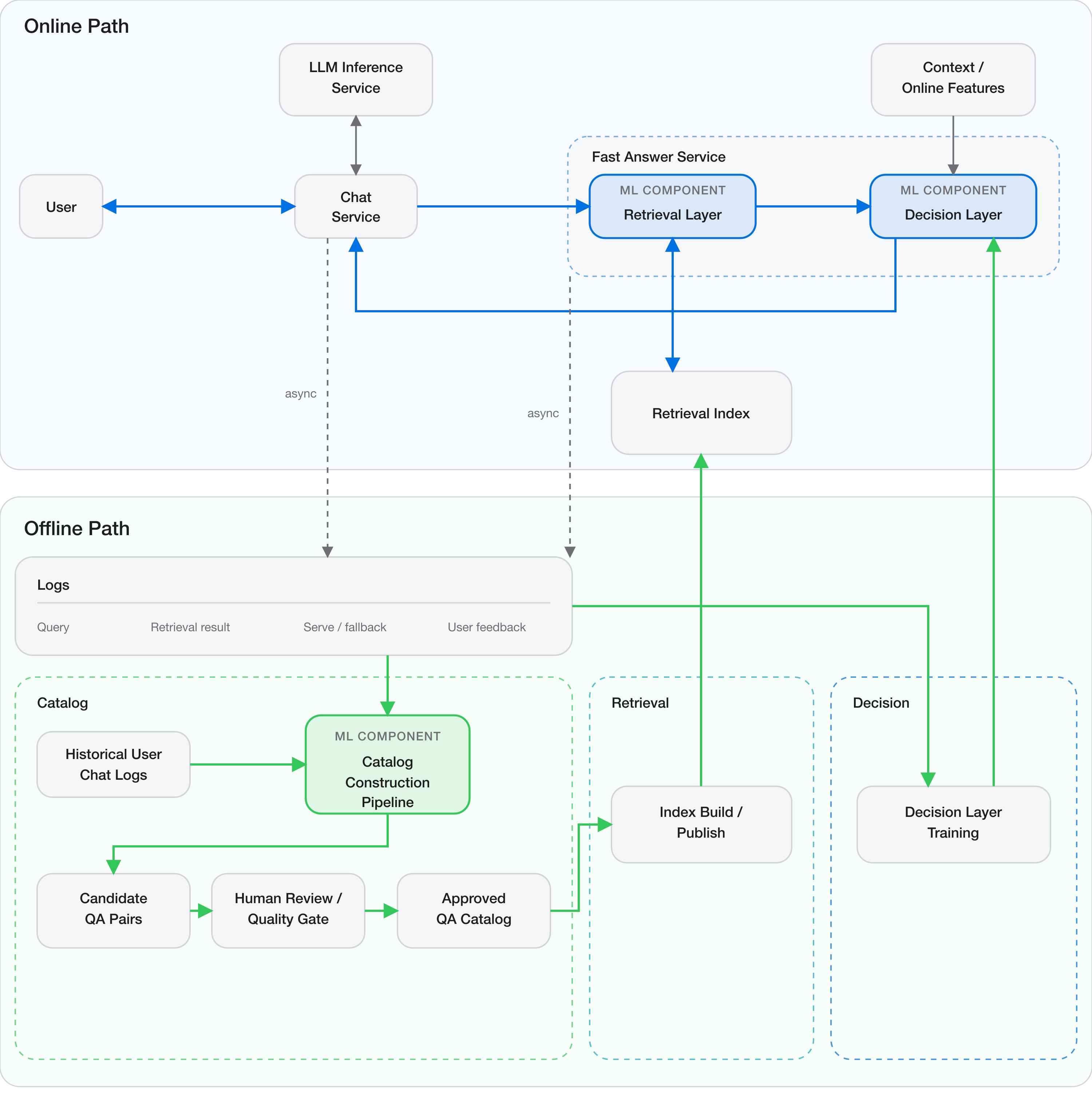
  <img src="/assets/diagrams/fast-answer-online-serving.png" alt="Online serving architecture of the Fast Answer system" />
</div>

<p><em>Figure 1. Online serving architecture of the Fast Answer system.</em></p>

<p>The Fast Answer Service itself should be stateless and deployed as a horizontally scalable service on Kubernetes. The Chat Service communicates with it through gRPC.</p>

<p>A stateless design allows the service to scale horizontally as traffic changes. Requests can be routed to any healthy replica without requiring session affinity, which simplifies load balancing and failure recovery.</p>

<p>Kubernetes is not the only deployment option. A serverless platform could provide automatic scaling with less operational overhead, while a fixed pool of virtual machines would be simpler to operate at small scale. However, the workload assumed here has both high sustained traffic and a strict p99 latency requirement. Maintaining a pool of warm replicas provides more predictable tail latency than relying on serverless instances that may experience cold starts.</p>

<p>I would therefore accept the additional operational complexity of Kubernetes in exchange for predictable warm capacity, horizontal scaling, rolling deployments, and controlled traffic rollout.</p>

<p>For communication between the Chat Service and Fast Answer Service, I would use gRPC rather than a JSON-based REST API. This is an internal, high-QPS service-to-service call where compact serialization and strongly typed interfaces are useful. The trade-off is additional schema management through Protocol Buffers and somewhat less convenient manual debugging compared with HTTP/JSON.</p>

<h3 id="32-retrieval-store-an-immutable-in-memory-catalog">3.2 Retrieval Store: An Immutable In-Memory Catalog</h3>

<p>The first version of Retrieval uses exact query matching. This makes the serving requirement substantially simpler than that of a general-purpose search system:</p>

\[\text{Normalized Query}
\rightarrow
\text{Catalog Entry}.\]

<p>A conventional design might place the Catalog behind Redis or another distributed key-value store. Redis would provide low-latency lookups, replication, and independent updates to the serving data. However, every lookup would still introduce an additional network hop and another dependency on the critical path.</p>

<p>Instead, I would first investigate whether the entire serving Catalog can be loaded directly into the memory of each Fast Answer Service replica.</p>

<p>Each Catalog version would be published as an immutable artifact. When a Fast Answer Service replica starts, it downloads the selected Catalog version and loads a mapping from normalized query to QA entry into memory. Retrieval then becomes a local hash-table lookup.</p>

<div class="language-text highlighter-rouge"><div class="highlight"><pre class="highlight"><code>Normalized Query
        ↓
In-Memory Hash Lookup
        ↓
QA Pair + Catalog Features
</code></pre></div></div>

<p>This design has several advantages for the current workload:</p>

<ul>
  <li>No network call is required for retrieval.</li>
  <li>Exact-match lookup is extremely cheap.</li>
  <li>Retrieval availability is coupled only to the health of the serving process itself.</li>
  <li>Every request is served against a known Catalog version.</li>
</ul>

<p>The main question is whether the Catalog is small enough to replicate in memory across all serving pods. The assumptions from Section 2 allow a rough upper-bound estimate.</p>

<p>The assumed human-review capacity is approximately 7,200 query candidates per day. Even if the initial Catalog construction runs for 30 days and every reviewed query is approved, the Catalog would contain at most:</p>

\[N_{\text{Catalog}}
\leq
7{,}200 \times 30
=
216{,}000\]

<p>entries.</p>

<p>The actual number would likely be smaller because some queries would fail eligibility review and some generated answers would fail answer review. For capacity planning, a Catalog of approximately <strong>200K entries</strong> is therefore a conservative initial estimate.</p>

<p>Suppose each entry contains approximately:</p>

<ul>
  <li>100 bytes for the normalized query</li>
  <li>2 KB for the prepared Fast Answer</li>
  <li>500 bytes for Catalog metadata and precomputed Decision features</li>
</ul>

<p>The serialized data is therefore roughly 2.6 KB per entry. Allowing approximately 2× overhead for strings, hash-table structures, and the in-memory representation gives a conservative estimate of roughly 5 KB per entry.</p>

<p>The resulting memory footprint is:</p>

\[200{,}000
\times
5\text{ KB}
\approx
1\text{ GB}.\]

<p>A roughly 1 GB Catalog can comfortably fit in the memory of each Fast Answer Service replica. Even allowing additional memory for the service process and Decision model, an instance with several gigabytes of memory should be sufficient.</p>

<p>Even if the human-review bottleneck were reduced and Catalog construction throughput improved by 10×, the same estimate would produce a Catalog of roughly 2 million entries, or about 10 GB per replica. That is still practical for a memory-optimized serving instance, so process-local replication would remain a reasonable choice at that scale.</p>

<h3 id="33-feature-serving">3.3 Feature Serving</h3>

<p>The Decision model uses two broad categories of features: Catalog-entry features and user features.</p>

<p>Catalog-entry features, such as historical uplift, answer age, feedback volume, and query frequency, are naturally associated with the retrieved QA entry. These features should therefore be packaged directly with the Catalog artifact.</p>

<p>A successful retrieval would return both the answer and its precomputed features:</p>

<div class="language-text highlighter-rouge"><div class="highlight"><pre class="highlight"><code>Catalog Entry
  ├── Query
  ├── Answer
  ├── Historical Uplift
  ├── Query Frequency
  ├── Catalog Age
  └── Other Precomputed Features
</code></pre></div></div>

<p>This avoids a separate feature-store lookup for data that changes relatively slowly and can be recomputed during Catalog publication.</p>

<p>User-level features are different. Features such as historical Fast Answer affinity or recent regeneration behavior may need to be fetched from an online feature store.</p>

<p>Adding this remote call, however, directly consumes part of the 200 ms p99 latency budget and introduces another dependency on the serving path.</p>

<p>I would therefore make the inclusion of user features conditional on their demonstrated predictive value.</p>

<p>The initial Decision model would first be evaluated using only features already available in the request and Catalog entry. I would add a remote user-feature lookup only if offline and online experiments show that the additional features produce a meaningful increase in Fast Answer serve rate under the same satisfaction constraint.</p>

<h3 id="34-decision-model-serving">3.4 Decision Model Serving</h3>

<p>The first learned Decision model described in <a href="/posts/chatgpt-fast-answer-1/">Part 1</a> does not require a large neural network. A logistic regression model, GBDT, or similarly lightweight model should be sufficient as an initial implementation.</p>

<p>For a model of this size, I would not deploy a separate model-serving system such as Triton or a dedicated inference microservice. Instead, the model would be loaded directly into the Fast Answer Service process and evaluated in-process.</p>

<div class="language-text highlighter-rouge"><div class="highlight"><pre class="highlight"><code>Retrieved QA + Features
        ↓
In-Process Decision Model
        ↓
Estimated Satisfaction Impact
        ↓
Decision Threshold
        ↓
Serve / Fall Back
</code></pre></div></div>

<p>This removes another network hop from the critical path and allows Decision inference to remain extremely cheap.</p>

<p>The trade-off is tighter coupling between the Decision model and the Fast Answer Service. Updating the model requires updating the artifact loaded by the service, and the model cannot scale independently from the rest of the Fast Answer Service.</p>

<p>For the current system, I would accept that trade-off. The model is small, and the Catalog itself already requires periodic version updates. Catalog and Decision model versions can therefore be packaged as part of the same serving release.</p>

<p>A serving bundle might look like:</p>

<div class="language-text highlighter-rouge"><div class="highlight"><pre class="highlight"><code>Fast Answer Release v42
  ├── Catalog v42
  ├── Catalog Features v42
  ├── Decision Model v17
  └── Decision Threshold v8
</code></pre></div></div>

<p>New pods can start with the new bundle while existing pods continue serving the previous version.</p>

<p>This also allows gradual rollout. Kubernetes can run both old and new replica sets simultaneously and shift traffic incrementally. If metrics regress, traffic can be shifted back to the previous version without rebuilding the Catalog or model.</p>

<h3 id="35-additional-considerations">3.5 Additional Considerations</h3>

<p>Fast Answer Service replicas should be deployed in the same regions as the Chat Service, with the same immutable serving bundle replicated across regions. This avoids adding a cross-region network hop to the latency-critical path.</p>

<p>Special care is also required to keep query-normalization logic consistent between the online and offline paths. A Catalog key produced by the offline pipeline must be identical to the key produced from the same query during online serving; otherwise, valid entries will become false misses.</p>

<p>The system also requires proper observability across the Chat Service, Fast Answer Service, Catalog, Decision model, and fallback path. I will discuss the monitoring and operational details in <a href="/posts/chatgpt-fast-answer-3/">Part 3</a>.</p>

<h2 id="4-offline-architecture">4. Offline Architecture</h2>

<p>The offline architecture has two responsibilities: constructing the QA Catalog and training the Decision model. The Catalog pipeline consumes historical chat logs to discover new QA opportunities and production feedback to identify existing entries that should be updated or deleted. Both offline pipelines process large-scale logs, but their final outputs are small enough to be packaged directly into the immutable serving bundle described in Section 3.</p>

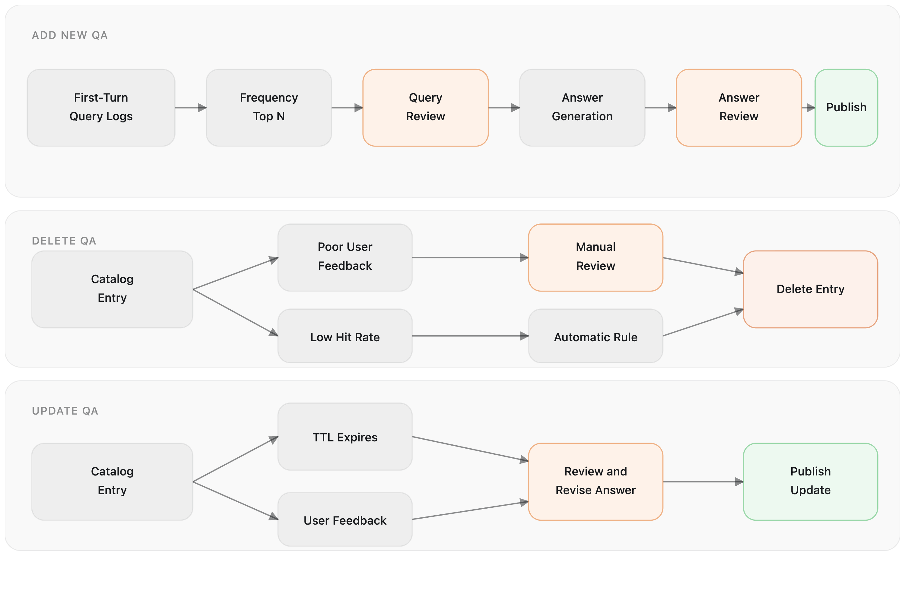
<div class="wide-diagram">
  <img src="/assets/diagrams/fast-answer-offline-pipeline.png?v=3" alt="Offline architecture of the Fast Answer system" />
</div>

<p><em>Figure 2. Offline architecture of the Fast Answer system.</em></p>

<h3 id="41-log-storage-and-incremental-aggregation">4.1 Log Storage and Incremental Aggregation</h3>

<p>Historical chat logs and production feedback are stored in object storage in a columnar format such as Parquet. Production feedback includes the served Catalog entry, entry-level traffic, thumbs-down feedback, and regeneration or retry behavior. Given the estimated scale of 25 billion queries for the initial 30-day backfill, Spark is a reasonable choice for distributed filtering, normalization, and aggregation.</p>

<p>The initial backfill should process these logs as daily partitions. This makes incremental updates to a 30-day sliding window straightforward: remove the oldest daily partition, add the newest one, and recompute the aggregate over the remaining 30 days. Each partition is processed independently, so the window can be refreshed without rescanning the complete raw history.</p>

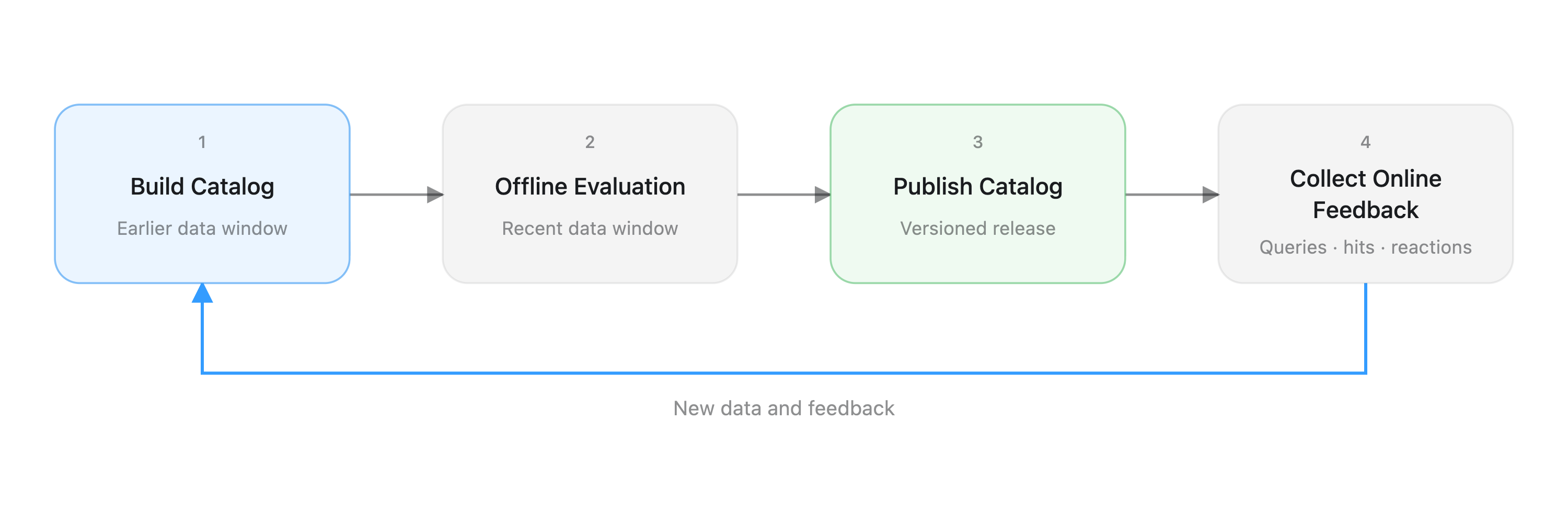
<p>The pipeline produces two derived datasets. Normalized query counts feed the path that discovers new Catalog entries, while entry-level feedback aggregates feed the path that proposes updates and deletions. This avoids rescanning approximately 25 billion raw records whenever the Catalog is rebuilt. The expensive raw-log processing happens only once per daily partition, while subsequent Catalog builds operate on much smaller aggregated representations.</p>

<p>I prefer this approach over maintaining a single continuously updated global frequency table. Daily aggregates can remain immutable, which makes backfills and recovery simpler. If processing for one day is incorrect, that partition can be recomputed independently and the 30-day aggregate rebuilt from the corrected result.</p>

<p>This composition works naturally for additive statistics such as query counts and feedback counts. More complex statistics may require additional mergeable state. Query frequency is the primary signal for discovering new Catalog entries, while production feedback provides the primary signals for updating or deleting existing entries.</p>

<h3 id="42-candidate-generation-and-human-review">4.2 Candidate Generation and Human Review</h3>

<p>Both offline paths produce candidates for human review. As estimated in Section 2, the assumed review capacity is approximately 7,200 candidates per day, so each path must reduce its aggregated data to a small set of high-value candidates.</p>

<h4 id="add-candidates">Add Candidates</h4>

<p>The 30-day query aggregation still produces far more queries than humans can review. The initial system can keep candidate generation simple: queries already covered by the Catalog are removed, basic eligibility rules filter obvious non-candidates, and the remaining queries are ranked primarily by traffic frequency.</p>

<div class="language-text highlighter-rouge"><div class="highlight"><pre class="highlight"><code>30-Day Query Frequency
        ↓
Remove Existing Catalog Entries
        ↓
Eligibility Rules
        ↓
Rank by Expected Coverage Gain
        ↓
Top Candidates within Review Budget
</code></pre></div></div>

<h4 id="update-and-delete-candidates">Update and Delete Candidates</h4>

<p>The second path aggregates production feedback for existing Catalog entries. Entries with unusually negative feedback, increasing regeneration or retry behavior, or freshness concerns become update candidates. Entries with persistently low traffic or severe quality problems can become delete candidates.</p>

<p>These rules do not mutate the Catalog directly. They produce a prioritized set of update and delete candidates that joins the add candidates at the human-review stage.</p>

<p>At this point, the problem is no longer a distributed-compute bottleneck. Spark may process hundreds of millions of records upstream, but the combined output of both paths should be only thousands of review candidates per day.</p>

<p>The selected candidates can then be written to PostgreSQL, which serves as the backend for the internal review workflow. A relational database is appropriate here because the workload is relatively small and the important requirements are transactional state transitions and auditability rather than large-scale analytical processing.</p>

<p>The review workflow depends on the proposed action:</p>

<div class="language-text highlighter-rouge"><div class="highlight"><pre class="highlight"><code>PENDING_REVIEW
  ├── ADD_APPROVED → ANSWER_GENERATING → ANSWER_REVIEW
  ├── UPDATE_APPROVED → ANSWER_GENERATING → ANSWER_REVIEW
  └── DELETE_APPROVED → DELETED
</code></pre></div></div>

<p>PostgreSQL also becomes the source of truth for the Catalog management workflow. The online serving system does not query this database directly.</p>

<h3 id="43-catalog-mutation-and-answer-generation">4.3 Catalog Mutation and Answer Generation</h3>

<p>Approved add candidates proceed to answer generation. Update candidates may also require a newly generated answer, while approved delete candidates can be removed without generation. Because the upstream filtering stage reduces hundreds of millions of daily records to at most thousands of reviewed candidates, answer generation does not require a large dedicated serving system.</p>

<p>A durable task queue and a small pool of stateless generation workers should be sufficient. Each job contains the approved query or existing Catalog entry together with its generation configuration, and the result is written back to PostgreSQL for final human review.</p>

<p>The queue provides retry and failure isolation without coupling answer generation to the review application. Generation throughput can also be scaled independently if review capacity increases.</p>

<p>Once an answer for an add or update candidate passes review, the approved QA pair is written to the Catalog source of truth. An approved deletion marks the entry for exclusion from the next Catalog snapshot. The Catalog table would contain the information required to construct the serving artifact, including:</p>

<div class="language-text highlighter-rouge"><div class="highlight"><pre class="highlight"><code>Catalog Entry
  ├── Normalized Query
  ├── Fast Answer
  ├── Query Frequency
  ├── Historical Feedback
  ├── Catalog Age
  ├── Human Review Metadata
  └── Precomputed Decision Features
</code></pre></div></div>

<p>The Catalog itself remains mutable in PostgreSQL as entries are added, updated, or removed. Online serving, however, consumes only immutable snapshots built from an approved Catalog state.</p>

<h3 id="44-decision-model-training-pipeline">4.4 Decision Model Training Pipeline</h3>

<p>The Decision model is trained from the randomized experiment data described in <a href="/posts/chatgpt-fast-answer-1/">Part 1</a>. The raw experiment logs are stored in the same object-storage-based data platform used by the Catalog pipeline.</p>

<p>The scale requirements of data preparation and model training are different. Experiment logs may contain hundreds of millions of requests, so feature generation and training-dataset construction should use Spark. The actual Decision model, however, is expected to be a logistic regression, GBDT, or similarly lightweight model.</p>

<p>Distributed computation should handle data preparation, while the model itself can be trained on a single CPU machine using a library such as scikit-learn or XGBoost. There is little benefit in introducing distributed model-training infrastructure for a model this small.</p>

<p>After training, candidate thresholds are evaluated on randomized holdout data using the off-policy evaluation procedure described in Part 1:</p>

\[t^*
=
\arg\max_t
\operatorname{ServeRate}(t)
\quad
\text{s.t.}
\quad
\widehat{\Delta S}_{\text{OPE}}(t)
\ge
-\epsilon.\]

<p>The output of the training pipeline is therefore not only a model artifact but also the selected Decision threshold.</p>

<div class="language-text highlighter-rouge"><div class="highlight"><pre class="highlight"><code>Decision Model v17
Decision Threshold v8
</code></pre></div></div>

<p>Both are versioned independently so that a threshold can be changed without necessarily retraining the model.</p>

<h3 id="45-building-and-publishing-the-serving-bundle">4.5 Building and Publishing the Serving Bundle</h3>

<p>The Catalog and Decision pipelines eventually converge into a single release artifact.</p>

<div class="language-text highlighter-rouge"><div class="highlight"><pre class="highlight"><code>Approved Catalog
      ↓
Catalog Snapshot
      │
      ├──────────────┐
      │              │
Decision Model       │
Decision Threshold   │
      │              │
      └──────┬───────┘
             ↓
      Release Build
             ↓
Fast Answer Release v42
  ├── Catalog v42
  ├── Catalog Features v42
  ├── Decision Model v17
  ├── Decision Threshold v8
  └── Normalization Version v7
             ↓
Versioned Object Storage
             ↓
Kubernetes Rollout
</code></pre></div></div>

<p>The normalization version is included because offline Catalog construction and online Retrieval must produce exactly the same Catalog key for the same query. A normalization change must therefore be deployed together with a compatible Catalog snapshot.</p>

<p>The release artifact is immutable and stored in versioned object storage. When a new Fast Answer Service pod starts, it downloads the configured release, validates the artifact, loads the Catalog and Decision model into memory, and becomes ready to receive traffic only after initialization succeeds.</p>

<p>This allows old and new releases to coexist during a rollout. If the new release causes a regression, traffic can be moved back to pods running the previous immutable bundle.</p>

<p>This design deliberately moves complexity away from the online critical path. Catalog management, large-scale aggregation, model training, validation, and artifact construction all happen offline. The resulting online system only needs to load a verified bundle and execute local retrieval and lightweight Decision inference.</p>

<h2 id="5-failure-handling-and-capacity-validation">5. Failure Handling and Capacity Validation</h2>

<p>The Fast Answer path must remain optional from the Chat Service’s perspective. Each request receives a 200 ms hard timeout. A Fast Answer Service miss, error, or timeout causes the Chat Service to fall back to normal LLM generation, so a Fast Answer failure cannot disrupt the existing response path.</p>

<p>A circuit breaker provides protection against persistent failures. If the Fast Answer Service remains unhealthy, the Chat Service should temporarily stop calling it and route requests directly to LLM generation. On the serving side, a new pod should pass readiness checks only after it has downloaded, loaded, and validated its Catalog and Decision model artifacts.</p>

<p>Capacity should be determined through load testing rather than by guessing a replica count. The sustainable QPS of one fully initialized pod should be measured under a realistic request mix and verified against the 200 ms p99 latency budget. The required replica count can then be calculated as:</p>

\[N_{\text{replicas}}
=
\left\lceil
\frac{\text{QPS}_{\text{peak}}}{\text{QPS}_{\text{per replica}}}
\times
\text{Headroom Factor}
\right\rceil.\]

<p>The final load test should verify the approximately 30K QPS peak target from Section 2 with enough headroom for traffic spikes, pod failures, and rolling deployments.</p>

<h2 id="6-wrap-up">6. Wrap-up</h2>

<p>This post was intended as an architectural overview rather than a complete production design document. My goal was to identify the major infrastructure decisions that are specific to this system and reason about them from the scale and latency assumptions established earlier.</p>

<p>As a result, I intentionally left out general-purpose infrastructure concerns such as authentication, network configuration, access control, and other platform-level details that would be required in a real production system but are not particularly specific to Fast Answers.</p>

<p>There are also important questions around observability, deployment, experimentation, and ongoing operations that I have only briefly touched on here. These become especially important once the system is running in production and the Catalog, Decision model, and user traffic continuously change.</p>

<p>I will cover those topics in <a href="/posts/chatgpt-fast-answer-3/">Part 3</a>, focusing on how I would monitor, operate, and continuously improve the system after launch.</p>

<hr />

<p>If you have read this far, something in this post probably caught your interest. If you would like to know more about me, feel free to <a href="https://www.linkedin.com/in/jjonghu">connect with me on LinkedIn</a>.</p>]]></content><author><name>Jonghu</name></author><category term="system-design" /><category term="product" /><category term="openai" /><category term="architecture" /><summary type="html"><![CDATA[TL;DR This post designs how the ML system from Part 1 could be implemented in production. It focuses on the key production architecture decisions specific to a Fast Answer system. This is a four-part series: Part 0. Product Teardown and Related Work Part 1. Business Context and ML System Design Part 3. Operations and Continuous Improvement 1. Serving Requirements The requirements established in Part 1 can now be translated into system constraints: A Fast Answer must be served much faster than an LLM-generated response. A Fast Answer miss must not significantly increase the latency of the normal LLM response path. The system must support high QPS. A Fast Answer Service failure must not disrupt the existing ChatGPT response path. The QA catalog and Decision model must be updateable without disrupting serving. 2. Scale and Capacity Estimation 2.1 Online Serving Scale As discussed in Part 1, ChatGPT processed more than 2.5 billion messages per day by mid-2025. Averaged over a full day, this corresponds to approximately 29K messages per second: \[\frac{2.5\text{B messages}}{86{,}400\text{ seconds}} \approx 28.9\text{K messages/s}.\] However, Fast Answers in this design are evaluated only for the first turn of a new conversation, and OpenAI does not publicly report the average number of user messages per conversation. For capacity estimation, I assume an average of three user queries per conversation. The average Fast Answer request rate is therefore approximately: \[Q_{\text{first-turn, avg}} \approx \frac{28.9\text{K}}{3} \approx 9.6\text{K QPS}.\] This is only the daily average. Assuming peak traffic is approximately three times the average, the Fast Answer Service must handle: \[Q_{\text{peak}} \approx 3 \times 9.6\text{K} \approx 29\text{K QPS}.\] At a coarse level, this is a 20K+ QPS system. To operate safely under the estimated peak, however, the initial capacity target should be approximately 30K QPS and validated through load testing. 2.2 Latency SLO How should the SLO for the Fast Answer Service be defined? In Part 0, I observed that Fast Answers appeared with an end-to-end TTFT of roughly 600 ms. The service must satisfy two requirements. First, a cache hit must leave enough latency budget for the network, request routing, and client rendering to keep end-to-end TTFT near the observed value. Second, and more importantly, a cache miss should not significantly delay a request that eventually falls back to normal LLM generation. The Fast Answer TTFT can be decomposed as: \[\text{TTFT}_{\text{Fast}} = L_{\text{client/network}} +L_{\text{gateway/chat}} +L_{\text{Fast Answer Service}} +L_{\text{return/render}}\] An initial latency budget might look like this: Component Budget Client ↔ edge/network 100–200 ms Gateway / Chat Service 50–100 ms Fast Answer Service ≤ 200 ms p99 Response transport/rendering 50–100 ms Safety margin / tail variability Remaining budget To keep end-to-end TTFT around the observed 600 ms, the Fast Answer Service should initially target a p99 latency of 200 ms or less. Adding more than 200 ms of p99 latency to the fallback path is therefore assumed to be undesirable, making 200 ms p99 the initial latency budget for the Fast Answer Service. The exact number is a design assumption rather than a claim about OpenAI’s actual infrastructure. For a cache miss, the resulting latency is: \[\text{TTFT}_{\text{Fallback}} = L_{\text{Fast Answer Miss}} +\text{TTFT}_{\text{LLM}}\] As observed in Part 0, a normally generated response had a TTFT of roughly two seconds. To bound the additional delay on this path, the Chat Service should apply a hard timeout when calling the Fast Answer Service. If no answer arrives within 200 ms, it should immediately begin LLM generation. This keeps a Fast Answer miss from adding more than approximately 200 ms to the normal generation path. 2.3 Offline Data Processing Scale Online serving is only one side of the scale problem. Building the QA Catalog also requires an offline data-processing pipeline that can operate over historical traffic. The Catalog Construction Pipeline designed in Part 1 extracts first-turn queries from historical chat logs, calculates query frequencies, and promotes frequent queries that are likely to be suitable for Fast Answers into QA candidates. Under the earlier assumption of three user queries per conversation, the number of first-turn queries among 2.5 billion daily messages can be estimated as: \[N_{\text{first-turn/day}} \approx \frac{2.5\text{B}}{3} \approx 833\text{M queries/day}.\] Suppose the initial Catalog is built from the most recent 30 days of traffic. The initial backfill job must then process approximately: \[N_{\text{backfill}} \approx 833\text{M} \times 30 \approx 25\text{B queries}.\] This does not mean that every one of the 25 billion queries receives LLM generation or human review. Most records are reduced through inexpensive operations near the beginning of the pipeline: Historical Chat Logs ↓ First-Turn Filtering ↓ Query Normalization ↓ Distributed Aggregation ↓ Frequent Unique Queries ↓ Eligibility Filtering ↓ QA Candidates ↓ Human Review ↓ Answer Generation ↓ Human Review ↓ Approved QA Catalog The early stages perform relatively simple operations such as first-turn filtering, normalization, exact-query aggregation, and frequency counting. Repeated forms of the same normalized query can be reduced to one query and its frequency count: "What is quickselect?" "what is quickselect" "what is quickselect?" ↓ "what is quickselect" → 1,234,567 occurrences A frequency threshold and eligibility heuristics can then reduce the candidate set before human review. Raw-log processing may operate over billions of records, but expensive model inference and human review apply only to the much smaller candidate set that remains after filtering. The initial backfill should also be separated from recurring updates. The backfill processes billions of historical records once. Later Catalog updates do not need to rescan the complete history. An incremental pipeline can process only newly created first-turn queries and merge their counts into the existing query-frequency aggregates. The daily incremental input is approximately: \[N_{\text{incremental/day}} \approx 833\text{M queries}.\] If the system maintains a rolling window, query counts can be stored in daily partitions. Each update adds a new partition and removes an expired one, avoiding a complete rescan of the 30-day window. The main capacity requirements for the offline pipeline are therefore: Initial backfill: approximately 25B first-turn query records Daily incremental processing: approximately 833M new first-turn queries Distributed aggregation over normalized queries Incremental updates rather than repeated full-history scans These numbers are not estimates of OpenAI’s actual infrastructure. They are design assumptions used to determine the scale that the Catalog Construction Pipeline should support. 2.4 Human Review Capacity Even if distributed computation can process billions of queries, the final stages of Catalog Construction face a different bottleneck: human review. Human review cannot be scaled indefinitely by simply adding machines. The upstream candidate-generation pipeline should therefore optimize for selecting the most valuable candidates within a limited review budget, rather than producing as many candidates as possible. Human-review throughput can be approximated as: \[N_{\text{review/day}} = N_{\text{reviewers}} \times \frac{T_{\text{review/day}}}{T_{\text{review/item}}}.\] For example, suppose 20 reviewers each spend six hours per day actively reviewing queries, and an eligibility decision takes an average of 60 seconds: \[N_{\text{review/day}} = 20 \times \frac{6 \times 3{,}600}{60} = 7{,}200.\] Even when hundreds of millions of new first-turn queries arrive each day, human-review capacity may remain on the order of only thousands of items. This means that query frequency alone may not be sufficient for candidate generation. The pipeline should therefore adjust how aggressively it filters candidates to match the available human-review capacity. The exact filtering threshold is an operational parameter that should be chosen for the current situation. If human review becomes a bottleneck that keeps the Catalog too small to achieve a meaningful cache hit rate, the review stage could be optimized with a lightweight LLM Judge. The LLM Judge could handle straightforward cases automatically and route only difficult cases to human reviewers. I will not include this extension in the current design. 2.5 Design Targets The assumptions above can now be summarized as the initial design targets for the rest of this post: Component Scale / SLO Assumption Design Implication Fast Answer Service ~30K peak QPS Horizontally scalable online serving Fast Answer Service latency ≤ 200 ms p99 Strict timeout and lightweight request path Initial Catalog backfill ~25B first-turn queries Distributed batch processing Daily incremental input ~833M first-turn queries/day Incremental aggregation Human review capacity Thousands of items/day Aggressive candidate filtering and prioritization Catalog / Index update Periodic and incremental Versioned build and non-disruptive publish The online scale determines how the system must serve requests. The offline scale determines how the Catalog must be constructed. The human-review scale determines how aggressively candidate queries must be filtered and prioritized. The rest of this post will design the serving and infrastructure architecture against these constraints. 3. Online Serving Architecture The online serving path is designed around the constraints established in Section 2. The key design principle is to keep the Fast Answer path as simple as possible. Every additional network dependency or remote model call increases tail latency and creates another potential failure point. Since the current system uses exact-match retrieval and a lightweight Decision model, most of the serving logic can remain inside the Fast Answer Service itself. 3.1 Fast Answer Service Figure 1. Online serving architecture of the Fast Answer system. The Fast Answer Service itself should be stateless and deployed as a horizontally scalable service on Kubernetes. The Chat Service communicates with it through gRPC. A stateless design allows the service to scale horizontally as traffic changes. Requests can be routed to any healthy replica without requiring session affinity, which simplifies load balancing and failure recovery. Kubernetes is not the only deployment option. A serverless platform could provide automatic scaling with less operational overhead, while a fixed pool of virtual machines would be simpler to operate at small scale. However, the workload assumed here has both high sustained traffic and a strict p99 latency requirement. Maintaining a pool of warm replicas provides more predictable tail latency than relying on serverless instances that may experience cold starts. I would therefore accept the additional operational complexity of Kubernetes in exchange for predictable warm capacity, horizontal scaling, rolling deployments, and controlled traffic rollout. For communication between the Chat Service and Fast Answer Service, I would use gRPC rather than a JSON-based REST API. This is an internal, high-QPS service-to-service call where compact serialization and strongly typed interfaces are useful. The trade-off is additional schema management through Protocol Buffers and somewhat less convenient manual debugging compared with HTTP/JSON. 3.2 Retrieval Store: An Immutable In-Memory Catalog The first version of Retrieval uses exact query matching. This makes the serving requirement substantially simpler than that of a general-purpose search system: \[\text{Normalized Query} \rightarrow \text{Catalog Entry}.\] A conventional design might place the Catalog behind Redis or another distributed key-value store. Redis would provide low-latency lookups, replication, and independent updates to the serving data. However, every lookup would still introduce an additional network hop and another dependency on the critical path. Instead, I would first investigate whether the entire serving Catalog can be loaded directly into the memory of each Fast Answer Service replica. Each Catalog version would be published as an immutable artifact. When a Fast Answer Service replica starts, it downloads the selected Catalog version and loads a mapping from normalized query to QA entry into memory. Retrieval then becomes a local hash-table lookup. Normalized Query ↓ In-Memory Hash Lookup ↓ QA Pair + Catalog Features This design has several advantages for the current workload: No network call is required for retrieval. Exact-match lookup is extremely cheap. Retrieval availability is coupled only to the health of the serving process itself. Every request is served against a known Catalog version. The main question is whether the Catalog is small enough to replicate in memory across all serving pods. The assumptions from Section 2 allow a rough upper-bound estimate. The assumed human-review capacity is approximately 7,200 query candidates per day. Even if the initial Catalog construction runs for 30 days and every reviewed query is approved, the Catalog would contain at most: \[N_{\text{Catalog}} \leq 7{,}200 \times 30 = 216{,}000\] entries. The actual number would likely be smaller because some queries would fail eligibility review and some generated answers would fail answer review. For capacity planning, a Catalog of approximately 200K entries is therefore a conservative initial estimate. Suppose each entry contains approximately: 100 bytes for the normalized query 2 KB for the prepared Fast Answer 500 bytes for Catalog metadata and precomputed Decision features The serialized data is therefore roughly 2.6 KB per entry. Allowing approximately 2× overhead for strings, hash-table structures, and the in-memory representation gives a conservative estimate of roughly 5 KB per entry. The resulting memory footprint is: \[200{,}000 \times 5\text{ KB} \approx 1\text{ GB}.\] A roughly 1 GB Catalog can comfortably fit in the memory of each Fast Answer Service replica. Even allowing additional memory for the service process and Decision model, an instance with several gigabytes of memory should be sufficient. Even if the human-review bottleneck were reduced and Catalog construction throughput improved by 10×, the same estimate would produce a Catalog of roughly 2 million entries, or about 10 GB per replica. That is still practical for a memory-optimized serving instance, so process-local replication would remain a reasonable choice at that scale. 3.3 Feature Serving The Decision model uses two broad categories of features: Catalog-entry features and user features. Catalog-entry features, such as historical uplift, answer age, feedback volume, and query frequency, are naturally associated with the retrieved QA entry. These features should therefore be packaged directly with the Catalog artifact. A successful retrieval would return both the answer and its precomputed features: Catalog Entry ├── Query ├── Answer ├── Historical Uplift ├── Query Frequency ├── Catalog Age └── Other Precomputed Features This avoids a separate feature-store lookup for data that changes relatively slowly and can be recomputed during Catalog publication. User-level features are different. Features such as historical Fast Answer affinity or recent regeneration behavior may need to be fetched from an online feature store. Adding this remote call, however, directly consumes part of the 200 ms p99 latency budget and introduces another dependency on the serving path. I would therefore make the inclusion of user features conditional on their demonstrated predictive value. The initial Decision model would first be evaluated using only features already available in the request and Catalog entry. I would add a remote user-feature lookup only if offline and online experiments show that the additional features produce a meaningful increase in Fast Answer serve rate under the same satisfaction constraint. 3.4 Decision Model Serving The first learned Decision model described in Part 1 does not require a large neural network. A logistic regression model, GBDT, or similarly lightweight model should be sufficient as an initial implementation. For a model of this size, I would not deploy a separate model-serving system such as Triton or a dedicated inference microservice. Instead, the model would be loaded directly into the Fast Answer Service process and evaluated in-process. Retrieved QA + Features ↓ In-Process Decision Model ↓ Estimated Satisfaction Impact ↓ Decision Threshold ↓ Serve / Fall Back This removes another network hop from the critical path and allows Decision inference to remain extremely cheap. The trade-off is tighter coupling between the Decision model and the Fast Answer Service. Updating the model requires updating the artifact loaded by the service, and the model cannot scale independently from the rest of the Fast Answer Service. For the current system, I would accept that trade-off. The model is small, and the Catalog itself already requires periodic version updates. Catalog and Decision model versions can therefore be packaged as part of the same serving release. A serving bundle might look like: Fast Answer Release v42 ├── Catalog v42 ├── Catalog Features v42 ├── Decision Model v17 └── Decision Threshold v8 New pods can start with the new bundle while existing pods continue serving the previous version. This also allows gradual rollout. Kubernetes can run both old and new replica sets simultaneously and shift traffic incrementally. If metrics regress, traffic can be shifted back to the previous version without rebuilding the Catalog or model. 3.5 Additional Considerations Fast Answer Service replicas should be deployed in the same regions as the Chat Service, with the same immutable serving bundle replicated across regions. This avoids adding a cross-region network hop to the latency-critical path. Special care is also required to keep query-normalization logic consistent between the online and offline paths. A Catalog key produced by the offline pipeline must be identical to the key produced from the same query during online serving; otherwise, valid entries will become false misses. The system also requires proper observability across the Chat Service, Fast Answer Service, Catalog, Decision model, and fallback path. I will discuss the monitoring and operational details in Part 3. 4. Offline Architecture The offline architecture has two responsibilities: constructing the QA Catalog and training the Decision model. The Catalog pipeline consumes historical chat logs to discover new QA opportunities and production feedback to identify existing entries that should be updated or deleted. Both offline pipelines process large-scale logs, but their final outputs are small enough to be packaged directly into the immutable serving bundle described in Section 3. Figure 2. Offline architecture of the Fast Answer system. 4.1 Log Storage and Incremental Aggregation Historical chat logs and production feedback are stored in object storage in a columnar format such as Parquet. Production feedback includes the served Catalog entry, entry-level traffic, thumbs-down feedback, and regeneration or retry behavior. Given the estimated scale of 25 billion queries for the initial 30-day backfill, Spark is a reasonable choice for distributed filtering, normalization, and aggregation. The initial backfill should process these logs as daily partitions. This makes incremental updates to a 30-day sliding window straightforward: remove the oldest daily partition, add the newest one, and recompute the aggregate over the remaining 30 days. Each partition is processed independently, so the window can be refreshed without rescanning the complete raw history. The pipeline produces two derived datasets. Normalized query counts feed the path that discovers new Catalog entries, while entry-level feedback aggregates feed the path that proposes updates and deletions. This avoids rescanning approximately 25 billion raw records whenever the Catalog is rebuilt. The expensive raw-log processing happens only once per daily partition, while subsequent Catalog builds operate on much smaller aggregated representations. I prefer this approach over maintaining a single continuously updated global frequency table. Daily aggregates can remain immutable, which makes backfills and recovery simpler. If processing for one day is incorrect, that partition can be recomputed independently and the 30-day aggregate rebuilt from the corrected result. This composition works naturally for additive statistics such as query counts and feedback counts. More complex statistics may require additional mergeable state. Query frequency is the primary signal for discovering new Catalog entries, while production feedback provides the primary signals for updating or deleting existing entries. 4.2 Candidate Generation and Human Review Both offline paths produce candidates for human review. As estimated in Section 2, the assumed review capacity is approximately 7,200 candidates per day, so each path must reduce its aggregated data to a small set of high-value candidates. Add Candidates The 30-day query aggregation still produces far more queries than humans can review. The initial system can keep candidate generation simple: queries already covered by the Catalog are removed, basic eligibility rules filter obvious non-candidates, and the remaining queries are ranked primarily by traffic frequency. 30-Day Query Frequency ↓ Remove Existing Catalog Entries ↓ Eligibility Rules ↓ Rank by Expected Coverage Gain ↓ Top Candidates within Review Budget Update and Delete Candidates The second path aggregates production feedback for existing Catalog entries. Entries with unusually negative feedback, increasing regeneration or retry behavior, or freshness concerns become update candidates. Entries with persistently low traffic or severe quality problems can become delete candidates. These rules do not mutate the Catalog directly. They produce a prioritized set of update and delete candidates that joins the add candidates at the human-review stage. At this point, the problem is no longer a distributed-compute bottleneck. Spark may process hundreds of millions of records upstream, but the combined output of both paths should be only thousands of review candidates per day. The selected candidates can then be written to PostgreSQL, which serves as the backend for the internal review workflow. A relational database is appropriate here because the workload is relatively small and the important requirements are transactional state transitions and auditability rather than large-scale analytical processing. The review workflow depends on the proposed action: PENDING_REVIEW ├── ADD_APPROVED → ANSWER_GENERATING → ANSWER_REVIEW ├── UPDATE_APPROVED → ANSWER_GENERATING → ANSWER_REVIEW └── DELETE_APPROVED → DELETED PostgreSQL also becomes the source of truth for the Catalog management workflow. The online serving system does not query this database directly. 4.3 Catalog Mutation and Answer Generation Approved add candidates proceed to answer generation. Update candidates may also require a newly generated answer, while approved delete candidates can be removed without generation. Because the upstream filtering stage reduces hundreds of millions of daily records to at most thousands of reviewed candidates, answer generation does not require a large dedicated serving system. A durable task queue and a small pool of stateless generation workers should be sufficient. Each job contains the approved query or existing Catalog entry together with its generation configuration, and the result is written back to PostgreSQL for final human review. The queue provides retry and failure isolation without coupling answer generation to the review application. Generation throughput can also be scaled independently if review capacity increases. Once an answer for an add or update candidate passes review, the approved QA pair is written to the Catalog source of truth. An approved deletion marks the entry for exclusion from the next Catalog snapshot. The Catalog table would contain the information required to construct the serving artifact, including: Catalog Entry ├── Normalized Query ├── Fast Answer ├── Query Frequency ├── Historical Feedback ├── Catalog Age ├── Human Review Metadata └── Precomputed Decision Features The Catalog itself remains mutable in PostgreSQL as entries are added, updated, or removed. Online serving, however, consumes only immutable snapshots built from an approved Catalog state. 4.4 Decision Model Training Pipeline The Decision model is trained from the randomized experiment data described in Part 1. The raw experiment logs are stored in the same object-storage-based data platform used by the Catalog pipeline. The scale requirements of data preparation and model training are different. Experiment logs may contain hundreds of millions of requests, so feature generation and training-dataset construction should use Spark. The actual Decision model, however, is expected to be a logistic regression, GBDT, or similarly lightweight model. Distributed computation should handle data preparation, while the model itself can be trained on a single CPU machine using a library such as scikit-learn or XGBoost. There is little benefit in introducing distributed model-training infrastructure for a model this small. After training, candidate thresholds are evaluated on randomized holdout data using the off-policy evaluation procedure described in Part 1: \[t^* = \arg\max_t \operatorname{ServeRate}(t) \quad \text{s.t.} \quad \widehat{\Delta S}_{\text{OPE}}(t) \ge -\epsilon.\] The output of the training pipeline is therefore not only a model artifact but also the selected Decision threshold. Decision Model v17 Decision Threshold v8 Both are versioned independently so that a threshold can be changed without necessarily retraining the model. 4.5 Building and Publishing the Serving Bundle The Catalog and Decision pipelines eventually converge into a single release artifact. Approved Catalog ↓ Catalog Snapshot │ ├──────────────┐ │ │ Decision Model │ Decision Threshold │ │ │ └──────┬───────┘ ↓ Release Build ↓ Fast Answer Release v42 ├── Catalog v42 ├── Catalog Features v42 ├── Decision Model v17 ├── Decision Threshold v8 └── Normalization Version v7 ↓ Versioned Object Storage ↓ Kubernetes Rollout The normalization version is included because offline Catalog construction and online Retrieval must produce exactly the same Catalog key for the same query. A normalization change must therefore be deployed together with a compatible Catalog snapshot. The release artifact is immutable and stored in versioned object storage. When a new Fast Answer Service pod starts, it downloads the configured release, validates the artifact, loads the Catalog and Decision model into memory, and becomes ready to receive traffic only after initialization succeeds. This allows old and new releases to coexist during a rollout. If the new release causes a regression, traffic can be moved back to pods running the previous immutable bundle. This design deliberately moves complexity away from the online critical path. Catalog management, large-scale aggregation, model training, validation, and artifact construction all happen offline. The resulting online system only needs to load a verified bundle and execute local retrieval and lightweight Decision inference. 5. Failure Handling and Capacity Validation The Fast Answer path must remain optional from the Chat Service’s perspective. Each request receives a 200 ms hard timeout. A Fast Answer Service miss, error, or timeout causes the Chat Service to fall back to normal LLM generation, so a Fast Answer failure cannot disrupt the existing response path. A circuit breaker provides protection against persistent failures. If the Fast Answer Service remains unhealthy, the Chat Service should temporarily stop calling it and route requests directly to LLM generation. On the serving side, a new pod should pass readiness checks only after it has downloaded, loaded, and validated its Catalog and Decision model artifacts. Capacity should be determined through load testing rather than by guessing a replica count. The sustainable QPS of one fully initialized pod should be measured under a realistic request mix and verified against the 200 ms p99 latency budget. The required replica count can then be calculated as: \[N_{\text{replicas}} = \left\lceil \frac{\text{QPS}_{\text{peak}}}{\text{QPS}_{\text{per replica}}} \times \text{Headroom Factor} \right\rceil.\] The final load test should verify the approximately 30K QPS peak target from Section 2 with enough headroom for traffic spikes, pod failures, and rolling deployments. 6. Wrap-up This post was intended as an architectural overview rather than a complete production design document. My goal was to identify the major infrastructure decisions that are specific to this system and reason about them from the scale and latency assumptions established earlier. As a result, I intentionally left out general-purpose infrastructure concerns such as authentication, network configuration, access control, and other platform-level details that would be required in a real production system but are not particularly specific to Fast Answers. There are also important questions around observability, deployment, experimentation, and ongoing operations that I have only briefly touched on here. These become especially important once the system is running in production and the Catalog, Decision model, and user traffic continuously change. I will cover those topics in Part 3, focusing on how I would monitor, operate, and continuously improve the system after launch. If you have read this far, something in this post probably caught your interest. If you would like to know more about me, feel free to connect with me on LinkedIn.]]></summary><media:thumbnail xmlns:media="http://search.yahoo.com/mrss/" url="https://jonghu.github.io/assets/default-social-image.png" /><media:content medium="image" url="https://jonghu.github.io/assets/default-social-image.png" xmlns:media="http://search.yahoo.com/mrss/" /></entry><entry><title type="html">ChatGPT Fast Answers Part 1: Business Context and ML System Design</title><link href="https://jonghu.github.io/posts/chatgpt-fast-answer-1/" rel="alternate" type="text/html" title="ChatGPT Fast Answers Part 1: Business Context and ML System Design" /><published>2026-07-14T00:01:00-05:00</published><updated>2026-07-14T00:01:00-05:00</updated><id>https://jonghu.github.io/posts/chatgpt-fast-answer-1</id><content type="html" xml:base="https://jonghu.github.io/posts/chatgpt-fast-answer-1/"><![CDATA[<h2 id="tldr">TL;DR</h2>
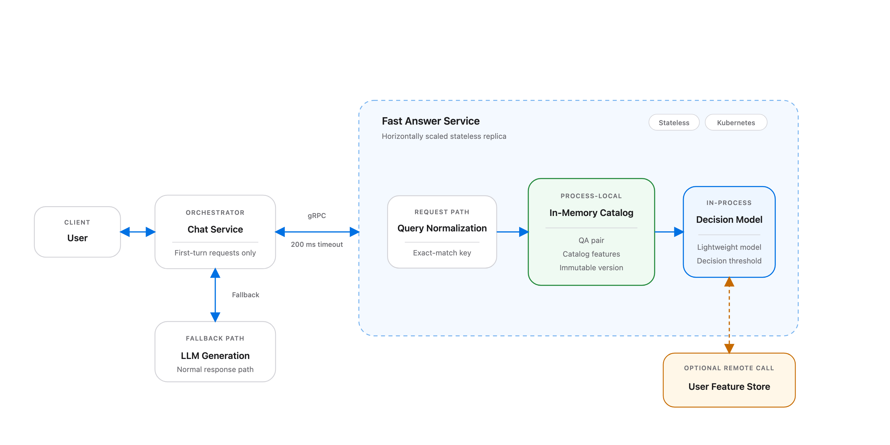
<ul>
  <li>Part 1 turns the product observations from <a href="/posts/chatgpt-fast-answer-0/">Part 0</a> into a business objective and an ML system design.</li>
  <li>This post is less about sophisticated model architectures and more about how to translate a business objective into concrete ML problems.</li>
</ul>

<p>This is a four-part series:<br />
<a href="/posts/chatgpt-fast-answer-0/">Part 0. Product Teardown and Related Work</a><br />
<a href="/posts/chatgpt-fast-answer-2/">Part 2. Production Architecture</a><br />
<a href="/posts/chatgpt-fast-answer-3/">Part 3. Operations and Continuous Improvement</a></p>

<h2 id="1-business-context--objective">1. Business Context &amp; Objective</h2>

<h3 id="11-business-objective">1.1 Business Objective</h3>

<p><a href="/posts/chatgpt-fast-answer-0/">Part 0</a> examined Fast answers from the outside: observable product behavior, related products, and relevant research. From this point on, I will imagine the reasoning that might have justified this project when OpenAI first began considering it internally. This may differ substantially from OpenAI’s actual thought process, but I wrote it for the fun of designing one product end to end.</p>

<p>A reasonable business objective for introducing Fast answers would be:</p>

<blockquote>
  <p><strong>Reduce inference cost and latency without degrading user satisfaction.</strong></p>
</blockquote>

<p>This section briefly justifies that objective, then defines the domain assumptions and metrics used throughout the rest of the design.</p>

<h3 id="12-traffic-scale-and-cacheable-opportunity">1.2 Traffic Scale and Cacheable Opportunity</h3>

<p>OpenAI’s internal data analysts and scientists were probably already studying the wide range of user queries. They would be able to estimate how often recurring information-seeking queries appear each day, what share of them are duplicates, and how many could be answered with a cached response. A question such as <em>Why is the sky blue?</em> has a stable answer over time, so a cached response may be sufficient.</p>

<p>ChatGPT operates at enormous scale. OpenAI’s report <em>How People Use ChatGPT</em> states that the product received 2.5 billion messages per day in 2025, with 24% classified as Seeking Information.<sup id="fnref:usage-paper"><a href="#fn:usage-paper" class="footnote" rel="footnote" role="doc-noteref">1</a></sup> This design applies Fast Answers only to the first query in a new chat, so the exact addressable traffic is unknown, but the scale is still informative.</p>

<p>The next question is how much of that traffic is repetitive and cacheable. Query frequencies in web search are often highly skewed, suggesting that a relatively small set of frequent queries may account for a meaningful share of traffic. ChatGPT may follow a different distribution, so applying a specific rule such as 80/20 would be questionable. Still, even 1% of the 600 million daily information-seeking messages would correspond to 6 million requests per day.</p>

<p>This motivates the working assumption that a relatively small prepared-answer catalog could cover a non-trivial share of eligible first-turn queries. Each successful cache hit replaces an otherwise necessary LLM generation, creating meaningful opportunities to reduce both inference cost and latency.</p>

<h3 id="13-estimating-potential-savings">1.3 Estimating Potential Savings</h3>

<p>A simple general expression for the resulting savings is:</p>

\[\begin{aligned}
\text{Daily Savings}
&amp;= N_{\text{new chats}} \times P_{\text{info}} \times P_{\text{eligible}\mid\text{info}} \\
&amp;\quad \times \text{HitRate} \\
&amp;\quad \times \left(C_{\text{generation}} - C_{\text{fast}}\right)
\end{aligned}\]

<ul>
  <li>$N_{\text{new chats}}$ is the unknown number of new conversations per day.</li>
  <li>$P_{\text{info}}$ is the unknown probability that the first query is information-seeking.</li>
  <li>$P_{\text{eligible}\mid\text{info}}$ is the unknown probability that an information-seeking first query is eligible for a Fast answer.</li>
  <li>$\text{HitRate}$ is determined by the system discussed in this series.</li>
  <li>$C_{\text{generation}}$ is the unknown internal generation cost.</li>
  <li>$C_{\text{fast}}$ is the much smaller lookup and serving cost.</li>
</ul>

<p>This expression does not include the increase in user satisfaction from lower latency or the additional value created by freeing GPU capacity.</p>

<h3 id="14-domain-assumptions">1.4 Domain Assumptions</h3>

<ul>
  <li>A meaningful portion of traffic is information-seeking and cacheable.</li>
  <li>Fast answers are applied only to the first query in a new chat, since a subsequent query implicitly demands context from the prior conversation.</li>
  <li>Returning a cached answer is always cheaper than generating a new answer.</li>
  <li>Some users may not be satisfied with a cached answer.</li>
  <li>The initial system supports English queries only.</li>
</ul>

<p>The decisions in the rest of this design will be based on these assumptions.</p>

<h3 id="15-metrics">1.5 Metrics</h3>

<p><strong>Primary metrics</strong></p>

<ul>
  <li>Inference cost reduction</li>
  <li>Latency reduction</li>
</ul>

<p><strong>Guardrail metrics</strong></p>

<ul>
  <li>User satisfaction, measured through negative feedback such as thumbs-down</li>
  <li>Regeneration or retry rate<sup id="fnref:regeneration-proxy"><a href="#fn:regeneration-proxy" class="footnote" rel="footnote" role="doc-noteref">2</a></sup></li>
</ul>

<h2 id="2-problem-formulation--ml-objective">2. Problem Formulation &amp; ML Objective</h2>

<h3 id="21-from-the-business-objective-to-fast-answer-serve-volume">2.1 From the Business Objective to Fast Answer Serve Volume</h3>

<p>The business objective can be written as:</p>

\[\begin{aligned}
\max_{\pi}\quad
&amp;\text{Cost Saving}_{\pi} + \alpha\,\text{Latency Saving}_{\pi} \\
\text{subject to}\quad
&amp;\text{Satisfaction}_{\pi}
\geq \text{Satisfaction}_{\text{LLM}} - \epsilon
\end{aligned}\]

<p>This objective means that the Fast Answer system $\pi$ should maximize cost and latency savings while ensuring that user satisfaction is not lower than when users receive LLM-generated answers. The $\epsilon$ term accounts for noise in the observed satisfaction metric.</p>

<p>As assumed above:</p>

\[\text{Cost}_{\text{Fast}} \ll \text{Cost}_{\text{LLM}},
\qquad
\text{Latency}_{\text{Fast}} \ll \text{Latency}_{\text{LLM}}\]

<p>Based on the domain assumptions above, serving an answer through the Fast Answer path always saves generation cost and latency. The cost and latency savings from each Fast Answer are therefore always positive. Let the combined saving per served Fast Answer be approximated as a constant $K &gt; 0$. Then:</p>

\[\text{Total Saving} \approx K \times N_{\text{Fast Answer Served}}\]

<p>Total saving is therefore approximately proportional to the number of Fast Answers served. The business objective can be approximated as:</p>

\[\begin{aligned}
\max\quad &amp;N_{\text{Fast Answer Served}} \\
\text{subject to}\quad
&amp;\text{User Satisfaction} \geq \text{Baseline} - \epsilon
\end{aligned}\]

<p>In plain language:</p>

<blockquote>
  <p><strong>Serve as many requests as possible with Fast Answers without degrading user satisfaction.</strong></p>
</blockquote>

<p>If cached answers could satisfy users unconditionally, always serving a Fast Answer would preserve satisfaction and maximize savings. In reality, Fast Answers cannot be served for every request:</p>

<ul>
  <li><strong>Catalog failure:</strong> no satisfactory, fresh, reusable answer exists.</li>
  <li><strong>Retrieval failure:</strong> such an answer exists, but the system does not retrieve it.</li>
  <li><strong>Decision fallback:</strong> the right answer is retrieved, but the policy falls back to LLM generation.</li>
</ul>

<p>The objective therefore remains maximizing the number of Fast Answers served subject to the satisfaction constraint. The serving volume is determined by how many opportunities the Catalog creates, how many Retrieval finds, and how many the Decision Policy converts into Fast Answers. Satisfaction remains a separate aggregate constraint on the overall serving policy.</p>

<h3 id="22-decomposing-fast-answer-serve-volume">2.2 Decomposing Fast Answer Serve Volume</h3>

<p>The next step is to decompose how the Fast Answer serve volume is produced. Ideally, the objective would be optimized end to end. However, dividing the problem into subproblems based on the funnel and failure cases implied by the domain knowledge above makes it much easier to solve. Although not optimizing the objective directly may introduce some loss, each individual problem can be solved more easily and accurately, potentially producing better overall performance. This type of staged approach is common in search and recommendation systems.</p>

<p>At least three events must occur in sequence:</p>

\[\begin{aligned}
A &amp;= \{\text{A satisfactory reusable answer exists in the catalog}\} \\
R &amp;= \{\text{The correct catalog answer is retrieved}\} \\
D &amp;= \{\text{The decision policy serves the retrieved answer}\}
\end{aligned}\]

<p>Under this sequential decomposition, the expected Fast Answer serve volume can be expressed as:</p>

\[\mathbb{E}\left[N_{\text{Fast Answer Served}}\right]
=
N_{\text{Total Traffic}}
\times
\underbrace{P(A)}_{\text{Catalog Coverage}}
\times
\underbrace{P(R \mid A)}_{\text{Retrieval Quality}}
\times
\underbrace{P(D \mid A,R)}_{\text{Decision Serve Rate}}\]

<p>From this decomposition, each of the three modules (Catalog, Retrieval, and Decision Policy) should have its own objective and metrics.</p>

<h3 id="23-module-level-objectives-and-metrics">2.3 Module-Level Objectives and Metrics</h3>

<h4 id="module-1--catalog-construction">Module 1 — Catalog Construction</h4>

<p><strong>Question</strong></p>

<blockquote>
  <p>Do we have a satisfactory reusable answer for this query?</p>
</blockquote>

<p><strong>Input → Output</strong></p>

<p>Historical query traffic → Prepared QA catalog</p>

<p><strong>Objective</strong></p>

<p>Maximize catalog coverage: the fraction of eligible traffic for which a satisfactory reusable answer exists.</p>

\[\max P(A)\]

<p><strong>Metrics</strong></p>

<ul>
  <li><strong>Primary:</strong> Traffic-weighted Coverage</li>
  <li><strong>Guardrails:</strong> Answer Quality, Freshness, Safety</li>
</ul>

<h4 id="module-2--retrieval">Module 2 — Retrieval</h4>

<p><strong>Question</strong></p>

<blockquote>
  <p>If a reusable answer exists, can we find the right one?</p>
</blockquote>

<p><strong>Input → Output</strong></p>

<p>User query + QA catalog → Best candidate QA pair</p>

<p><strong>Objective</strong></p>

\[\max P(R \mid A)\]

<p>Maximize the retrieval success rate, given that an appropriate answer exists.</p>

<p><strong>Metrics</strong></p>

<ul>
  <li><strong>Primary:</strong> Top-1 Compatibility or Precision@1</li>
  <li><strong>Secondary:</strong> Recall@K, False-match Rate</li>
</ul>

<h4 id="module-3--decision-policy">Module 3 — Decision Policy</h4>

<p><strong>Question</strong></p>

<blockquote>
  <p>If we found the right answer, should we actually serve it?</p>
</blockquote>

<p><strong>Input → Output</strong></p>

<p>User query + retrieved QA + available context → Serve Fast Answer / Fall back to LLM</p>

<p><strong>Objective</strong></p>

<p>The Decision Policy should maximize the Fast Answer serve rate while maintaining the satisfaction guardrail:</p>

\[\begin{aligned}
\max\quad &amp;\text{Fast Answer Serve Rate} \\
\text{subject to}\quad &amp;\Delta S \geq -\epsilon
\end{aligned}\]

<p>Here, $\Delta S$ represents the change in user satisfaction under the Fast Answer policy relative to always using LLM generation.</p>

<p>This may look similar to the global business objective, but it operates only after the upstream Catalog and Retrieval stages have succeeded. Under the earlier assumption that each Fast Answer produces approximately the same cost and latency saving, the remaining Decision problem reduces to identifying the requests for which that saving can be realized with an acceptable impact on user satisfaction.</p>

<p>This objective can be further reduced to a prediction problem. Let $x$ represent the information available to the Decision Policy, such as the user query, retrieved answer, and available user or contextual features. Let</p>

\[\pi(x) \in \{0,1\}\]

<p>denote the policy, where $\pi(x)=1$ means serving the Fast Answer and $\pi(x)=0$ means falling back to LLM generation.</p>

<p>For each request, define the expected satisfaction impact of serving the Fast Answer instead of the LLM as</p>

\[\tau(x)
=
\mathbb{E}\left[
S_{\text{Fast}}-S_{\text{LLM}}
\mid X=x
\right].\]

<p>The main modeling challenge is that $\tau(x)$ is not directly observable for an individual request, since the same request cannot simultaneously receive both a Fast Answer and an LLM response. <a href="#6-decision-layer">Section 6</a> discusses how randomized experimental data can be used to estimate it.</p>

<p>The Fast Answer serve rate is then</p>

\[\mathbb{E}[\pi(X)].\]

<p>Because requests with $\pi(X)=0$ still receive the baseline LLM response, the aggregate satisfaction change introduced by the policy is</p>

\[\mathbb{E}[\pi(X)\tau(X)].\]

<p>Therefore, the Decision Policy objective becomes</p>

\[\begin{aligned}
\max_{\pi}\quad
&amp;\mathbb{E}[\pi(X)] \\
\text{subject to}\quad
&amp;\mathbb{E}[\pi(X)\tau(X)] \geq -\epsilon.
\end{aligned}\]

<p>Using Lagrangian relaxation, this can be written as</p>

\[\mathcal{L}(\pi,\lambda)
=
\mathbb{E}[\pi(X)]
+\lambda\left(\mathbb{E}[\pi(X)\tau(X)]+\epsilon\right),
\qquad \lambda \geq 0.\]

<p>Rearranging,</p>

\[\mathcal{L}(\pi,\lambda)
=
\mathbb{E}\left[\pi(X)(1+\lambda\tau(X))\right]
+\lambda\epsilon.\]

<p>For a fixed $\lambda$, the optimal policy is therefore</p>

\[\pi(x)
=
\begin{cases}
1, &amp; \text{if } 1+\lambda\tau(x)&gt;0, \\
0, &amp; \text{if } 1+\lambda\tau(x)&lt;0.
\end{cases}\]

<p>The original constrained optimization problem can therefore be implemented by estimating $\tau(x)$, the expected satisfaction impact of serving a Fast Answer instead of an LLM response, and choosing a threshold that maximizes the serve rate while satisfying the aggregate satisfaction constraint.</p>

<p>The Lagrange multiplier $\lambda$ controls the trade-off between serving more Fast Answers and preserving satisfaction. In practice, rather than explicitly optimizing $\lambda$, I would sweep the decision threshold on held-out experimental data and choose the lowest threshold whose estimated satisfaction delta still satisfies the guardrail. This yields the highest Fast Answer serve rate among policies that meet the satisfaction constraint.</p>

<p><strong>Metrics</strong></p>

<ul>
  <li><strong>Primary:</strong> Fast Answer Serve Rate</li>
  <li><strong>Guardrail:</strong> Satisfaction Delta</li>
</ul>

<h3 id="24-connecting-module-objectives-to-business-value">2.4 Connecting Module Objectives to Business Value</h3>

<p>The complete relationship can be summarized with one equation:</p>

\[\begin{aligned}
\mathbb{E}\left[N_{\text{Fast Answer Served}}\right]
= N
&amp;\times \underbrace{P(A)}_{\text{Catalog Coverage}} \\
&amp;\times \underbrace{P(R \mid A)}_{\text{Retrieval Success}} \\
&amp;\times \underbrace{P(D \mid A,R)}_{\text{Decision Serve Rate}}
\end{aligned}\]

<p>and:</p>

\[\mathbb{E}[\text{Business Saving}]
\approx K \times \mathbb{E}\left[N_{\text{Fast Answer Served}}\right]\]

<p>The logic is therefore:</p>

\[\begin{gathered}
\uparrow\text{Catalog Coverage},\quad
\uparrow\text{Retrieval Quality},\quad
\uparrow\text{Decision Serve Rate} \\
\Downarrow \\
\uparrow\text{Fast Answer Serve Volume} \\
\Downarrow \\
\uparrow\text{Cost and Latency Saving} \\
\text{subject to Satisfaction Delta} \geq -\epsilon
\end{gathered}\]

<p>This explains why optimizing each module’s local objective should improve the global business objective.</p>

<p>The reason to define this framework before designing the individual modules is that it provides debuggability and prioritization. If the complete system underperforms, module-level objectives and metrics make it possible to isolate the root cause and decide where further investment will have the greatest impact.</p>

<p>Additionally, each module does not need to be a fancy deep-learning model. For each module, define what goes in, what comes out, what should be optimized, and how success is measured.</p>

<h2 id="3-high-level-architecture">3. High-Level Architecture</h2>

<h3 id="31-high-level-architecture">3.1 High-Level Architecture</h3>

<p><img src="/assets/diagrams/fast-answer-architecture.png" alt="High-level architecture of the Fast Answer system" /></p>

<p><em>Figure 1. High-level architecture of the Fast Answer system.</em></p>

<p>The high-level architecture is divided into two paths. The first is the online path that handles user requests. When a request reaches the Chat Service, it calls the Fast Answer Service first for the initial query in a chat. If the Fast Answer Service returns an answer, the Chat Service immediately sends it back to the user. Otherwise, it invokes LLM generation.</p>

<p>Within the Fast Answer Service, the Retrieval Layer first searches a prebuilt index for a candidate QA pair. The Decision Layer then determines whether that candidate should be shown. It combines the candidate QA pair with context from the online feature store to make the final decision. Each stage must also log its outputs asynchronously so that the data can later support analysis and model training.</p>

<p>The offline path uses accumulated logs to build the QA catalog. An automated pipeline extracts candidate QA pairs, which pass through a review process before entering the final catalog. This process may add new QA pairs or update and remove existing ones. A periodic job then builds the retrieval index from the catalog. The Decision Layer should also be continuously retrained on newly collected data and updated when a new model is ready.</p>

<p>A more complete system would require additional discussion of retrieval-model training, feature-store pipelines, deployment, A/B testing, and other production concerns. The diagram shows only the components most central to the ML design. The technical implementation and operational details will be covered in later posts.</p>

<h3 id="32-heuristic-based-v0">3.2 Heuristic-Based V0</h3>

<p>Suppose the first Fast Answer system is implemented and launched from this architecture. Because the Catalog, Retrieval, and Decision layers are modularized, the work can be divided across the available team. If I had to build it alone, however, the first version would exclude complex ML components and focus on getting the complete system running. Section 2 defines each module’s objective as an ML problem, but the launch version does not necessarily need an ML model.</p>

<p>For example, the Catalog module could use exact matching to find high-frequency queries, generate LLM answers for them, and send those answers through manual review. Retrieval could use an index built for exact matching. After upstream eligibility checks pass, an experiment assignment layer could randomly assign a small fraction of traffic to either a Fast Answer or LLM generation. None of these approaches is sophisticated, but together they provide a set of heuristics that should behave reasonably well for an initial launch.</p>

<h3 id="33-what-should-we-improve-next">3.3 What Should We Improve Next?</h3>

<p>Suppose the system is now running with heuristic-based modules. The next step is to experiment on a small fraction of traffic, verify that the system and business metrics are healthy, and confirm that the required logs are being collected correctly. Once those checks pass, each module can be improved against the objectives defined earlier.</p>

<p>If resources allow only one module to be improved first, I would choose the Decision Layer. The Catalog should already work reasonably well because every entry passes through manual review, even though that review is expensive. Exact-match Retrieval is deliberately high precision. The largest uncertainty immediately after launch is therefore: <em>Should this retrieved answer actually be shown?</em> This decision sits closest to the satisfaction guardrail. Because the V0 experiment assignment is randomized at the chat-session level, it also provides controlled comparison data for learning a policy.</p>

<p>Using this randomized data to train a learned Decision Layer would make it possible to incorporate user context and make better serving decisions. For example, the system could show more Fast Answers to users who are usually satisfied with them.</p>

<p>The Catalog would be my second priority. Automating part of the manual-review process is likely to have high ROI. It would reduce review costs, and the work required for automation would force the team to define the intended behavior of Fast Answers more precisely. The knowledge and data accumulated during V0 operation would make that definition easier.</p>

<p>Retrieval would come last. Once the Catalog work has clarified the product objective, the system could begin moving from exact matching toward semantic matching. This ordering follows from the example in <a href="/posts/chatgpt-fast-answer-0/#33-retrieval">Part 0</a>, where a general-purpose text embedder was not aligned with answer equivalence.</p>

<p>The remainder of this post focuses on the modeling design for the three components, with particular emphasis on the Decision Policy as the first learned optimization target. Even when the Catalog or Retrieval modules remain heuristic-based, the discussion will cover what data should be used to evaluate and launch them. It will also briefly introduce possible approaches for more advanced modeling.</p>

<h2 id="4-catalog">4. Catalog</h2>

<p>The Catalog system is essentially a system that extracts information satisfying a particular set of conditions from chat logs offline and stores only a selected subset. Those conditions may require a query to occur frequently, ask for information, support a stable answer, and satisfy other product requirements.</p>

<p>This is a well-known industry pattern. Structurally, this resembles offline indexing and knowledge-base construction systems: extract information useful for a specific serving objective, filter it, and publish it in a retrievable form. Examples include search indexing and ChatGPT’s recently introduced improved Memory feature.<sup id="fnref:chatgpt-memory"><a href="#fn:chatgpt-memory" class="footnote" rel="footnote" role="doc-noteref">3</a></sup></p>

<h3 id="41-catalog-lifecycle">4.1 Catalog Lifecycle</h3>

<p>As discussed above, I would begin with a heuristic-based system. The full lifecycle would look like this:</p>

<p><img src="/assets/diagrams/catalog-lifecycle.png" alt="Lifecycle of the Fast Answer catalog" /></p>

<p><em>Figure 2. Build the catalog, evaluate it on recent data, publish it, collect online feedback, and repeat.</em></p>

<p>The sequence is straightforward. Build the catalog from a slightly older data window, evaluate it offline on recent data, publish it, collect feedback from production, and rebuild it with new data. The iteration cadence depends on how frequently the query distribution changes. It would be better to iterate more frequently at the beginning. Once the catalog has converged to some degree, a longer iteration cycle should be acceptable.</p>

<h3 id="42-heuristic-based-catalog-build">4.2 Heuristic-Based Catalog Build</h3>

<p>Catalog construction has three paths: adding new QA pairs, deleting existing QA pairs, and updating existing answers.</p>

<p><img src="/assets/diagrams/catalog-management-paths.png" alt="Three paths for adding, deleting, and updating catalog entries" /></p>

<p><em>Figure 3. The three paths in the heuristic-based catalog construction system.</em></p>

<h4 id="adding-new-qa-pairs">Adding New QA Pairs</h4>

<p>The first path adds a new QA pair through three stages:</p>

<ol>
  <li>Query extraction and manual review</li>
  <li>Answer generation and manual review</li>
  <li>Catalog publishing</li>
</ol>

<p>Query extraction begins by pulling a list of first-turn queries from chat logs. The system counts them using exact matching and selects the top $N$ most frequent queries. A human then filters this list for information-seeking queries.</p>

<p>Next, a separate LLM generates an answer for each approved query. Reusing an answer from existing chat logs would be risky for two reasons. First, the answer may contain personalized information because the model may have used memory. Second, a Fast Answer may require its own target length and tone.</p>

<p>Generating a fresh answer is therefore a reasonable choice. The generated answer also passes through manual review. An approved QA pair is then published to the catalog.</p>

<h4 id="deleting-qa-pairs">Deleting QA Pairs</h4>

<p>The second path removes QA pairs. Many heuristic rules are possible, but two signals are especially important:</p>

<ul>
  <li>Poor user feedback</li>
  <li>Low hit rate</li>
</ul>

<p>An entry with consistently poor user feedback can be sent through manual review and deleted. An entry with sufficiently low traffic can be removed automatically when catalog maintenance or review cost matters.</p>

<h4 id="updating-qa-pairs">Updating QA Pairs</h4>

<p>The third path updates QA pairs. The clearest reason to update an entry is that its answer has become outdated, but automatically detecting this is difficult. A simple solution is to assign a TTL to each answer and review it when the TTL expires. User feedback can also trigger manual review and an answer update.</p>

<p>Updating a question does not need a separate path. In practice, changing a question is equivalent to deleting the old entry and adding a new one.</p>

<p>The design above assumes that every manual review is performed by a person. An LLM Judge could make this process faster, but simply prompting an LLM would not be sufficient. The process described in <a href="/posts/llm-as-a-judge-in-practice/">LLM-as-a-Judge in Practice</a> provides a better way to build one, so I will not repeat that discussion here.</p>

<h3 id="43-offline-evaluation">4.3 Offline Evaluation</h3>

<p>Even a heuristic-based catalog requires evaluation before deployment. As discussed in Section 2, the Catalog’s role is to maximize coverage of QA pairs eligible for Fast Answers. The evaluation split should therefore be time-based: build the catalog from historical data, then measure traffic-weighted catalog coverage on more recent data.</p>

<p>The metric can be written as:</p>

\[\text{Traffic-Weighted Coverage}
=
\frac{
\sum_{q \in Q_{\mathrm{recent}}} n_q
\cdot \mathbb{1}[q \text{ has a satisfactory reusable answer in the catalog}]
}{
\sum_{q \in Q_{\mathrm{recent}}} n_q
}\]

<p>Here, $n_q$ is the number of times query $q$ appears in the recent evaluation window.</p>

<p>Answer quality, freshness, and safety are the guardrail metrics. The catalog should be independently re-audited on the evaluation date rather than evaluated using the same labels that were used to approve entries. The resulting audit can measure a pass rate for each dimension:</p>

\[\text{Pass Rate}_d
=
\frac{
\sum_{a \in C} \mathbb{1}[a \text{ passes dimension } d]
}{|C|},
\qquad
d \in \{\text{quality},\text{freshness},\text{safety}\}\]

<p>The audit labels could use a Likert scale, but I would recommend binary labels. The reason is discussed in <a href="/posts/llm-as-a-judge-in-practice/#make-evaluation-as-simple-as-possible">LLM-as-a-Judge in Practice</a>.</p>

<p>This produces a heuristic-based catalog system that can still be evaluated with data and deployed with a reasonable degree of confidence.</p>

<h3 id="44-online-evaluation">4.4 Online Evaluation</h3>

<p>The online evaluation of the Catalog asks one question:</p>

<blockquote>
  <p><strong>Is the published catalog creating the opportunities we expected under actual live traffic?</strong></p>
</blockquote>

<p>The first metric is Online Catalog Coverage:</p>

\[\text{Online Catalog Coverage}
=
\frac{
\sum_{q \in Q_{\mathrm{live}}} n_q
\cdot \mathbb{1}[q \text{ has an entry in the published catalog}]
}{
\sum_{q \in Q_{\mathrm{live}}} n_q
}\]

<p>This checks whether the coverage measured offline on a historical window is maintained under actual production traffic.</p>

<p>The second metric is the coverage gain from a newly published catalog:</p>

\[\Delta \text{Coverage}
=
\text{Coverage}_{\mathrm{new}}
-
\text{Coverage}_{\mathrm{old}}\]

<p>This measures how much additional traffic the new catalog covers relative to the previous version. It also shows whether newly added QA pairs are actually receiving traffic. If many entries are rarely used, the Catalog Construction process may be inefficient.</p>

<p>Finally, downstream feedback should be aggregated at the catalog-entry level. For every catalog answer that is actually served, useful signals include:</p>

<ul>
  <li>Thumbs-down feedback</li>
  <li>Regeneration or retry</li>
</ul>

<p>These signals can trigger the review, update, or deletion paths described above.</p>

<h3 id="45-advanced-directions">4.5 Advanced Directions</h3>

<p>A more advanced catalog system should be able to answer the following questions:</p>

<ul>
  <li>Can query extraction become more robust than simple frequency ranking?</li>
  <li>How can answer generation use user feedback to update answers automatically and improve user satisfaction?</li>
  <li>How far can manual review be reduced? Can the LLM Judge become reliable enough that humans review only hard samples?</li>
  <li>How frequently should the catalog be updated to return stable answers?</li>
</ul>

<h2 id="5-retrieval">5. Retrieval</h2>

<p>Retrieval deliberately uses exact matching to keep the system complexity low. When a query arrives, the system looks it up in the catalog. If the exact same query exists, it retrieves the corresponding answer.</p>

<p>From the perspective of query matching, this provides effectively perfect precision. That does not mean the retrieved answer will always satisfy the user. Answer satisfaction still depends on the quality of the QA curation performed by the Catalog system.</p>

<p>Because exact-match Retrieval introduces no additional modeling uncertainty, I would not build a separate ML evaluation pipeline for Retrieval in V0. Basic correctness and index-consistency checks would still be required.</p>

<p>If the system is later extended to retrieve answers for semantically similar queries, see the Retrieval discussion in <a href="/posts/chatgpt-fast-answer-0/#33-retrieval">Part 0</a>.</p>

<h2 id="6-decision-layer">6. Decision Layer</h2>

<h3 id="61-collecting-training-data">6.1 Collecting Training Data</h3>

<p>The first problem is that the expected satisfaction impact defined in Section 2 cannot be observed directly for an individual request:</p>

\[\tau(x)
=
\mathbb{E}\left[
S_{\text{Fast}}-S_{\text{LLM}}
\mid X=x
\right].\]

<p>The same request cannot simultaneously receive both a Fast Answer and an LLM response. V0 should therefore randomize traffic only after it passes the upstream eligibility checks:</p>

<div class="language-text highlighter-rouge"><div class="highlight"><pre class="highlight"><code>Retrieved Valid QA
        ↓
Eligibility Gate
        ↓
Experiment Assignment
   ├── Fast Answer
   └── LLM
</code></pre></div></div>

<p>For each assigned request, the system should collect:</p>

<ul>
  <li>$x$: the query, retrieved QA pair, catalog metadata, and available user or contextual features</li>
  <li>Treatment assignment: Fast Answer or LLM</li>
  <li>Satisfaction outcomes, including thumbs-down and regeneration or retry</li>
  <li>A composite satisfaction label, if needed</li>
</ul>

<p>Randomization makes the two groups comparable and provides the counterfactual evidence needed to estimate the satisfaction impact of Fast Answers.</p>

<p>Even after the Decision Policy is upgraded from V0 to V1, a small fraction of eligible traffic should remain randomized. This continuously provides unbiased data that can be used for future model training and evaluation.</p>

<h3 id="62-estimating-satisfaction-impact">6.2 Estimating Satisfaction Impact</h3>

<p>The simplest approach is to fit two outcome models (T-learner). Let $T$ denote the randomized treatment assignment:</p>

\[\widehat{S}_{F}(x)
=
\mathbb{E}[S \mid T=\text{Fast}, X=x]\]

\[\widehat{S}_{L}(x)
=
\mathbb{E}[S \mid T=\text{LLM}, X=x].\]

<p>The estimated satisfaction impact is then:</p>

\[\widehat{\tau}(x)
=
\widehat{S}_{F}(x)-\widehat{S}_{L}(x).\]

<p>This is essentially an uplift estimation problem. There is no need to begin with a complex model. Logistic regression, a GBDT, or a small MLP would all be reasonable candidates.</p>

<p>The training pipeline may be sophisticated, but online inference must remain cheap. The Decision Layer sits on the latency-critical path:</p>

\[L_{\text{Fast}}
=
L_{\text{Retrieval}}
+L_{\text{Decision}}
+L_{\text{Serving}}.\]

<p>If $L_{\text{Decision}}$ becomes large, the Decision Layer undermines the latency advantage that gives Fast Answers their value.</p>

<h3 id="63-features">6.3 Features</h3>

<p>The first model would not use query or answer text directly. Supporting text inputs would introduce additional complexity, including offline and online embedding pipelines. Simple aggregation-based features are a better starting point.</p>

<p>Whenever possible, features should be available without an additional remote call. The first version should rely primarily on query, answer, catalog, and user information that is already available or retrieved as part of an existing call.</p>

<p><strong>Catalog entry features</strong></p>

<ul>
  <li>Historical uplift for each query</li>
  <li>Answer length</li>
  <li>Query frequency</li>
  <li>Catalog entry age</li>
  <li>Time since the last human review</li>
  <li>Historical feedback volume</li>
  <li>Historical satisfaction variance</li>
  <li>Answer update count</li>
</ul>

<p><strong>User features</strong></p>

<ul>
  <li>Historical Fast Answer negative-feedback rate</li>
  <li>Historical LLM negative-feedback rate</li>
  <li>Smoothed user-level uplift</li>
  <li>Randomized-history sample count</li>
  <li>Average number of queries per conversation</li>
  <li>Language or locale</li>
  <li>Account tenure</li>
  <li>Recent Fast Answer feedback</li>
  <li>Recent regeneration behavior</li>
</ul>

<p>Fast Answer affinity should be measured relative to the user’s LLM baseline rather than from Fast Answer feedback alone:</p>

\[\text{Fast Answer Affinity}(u)
\approx
S_{\text{Fast}}(u)-S_{\text{LLM}}(u).\]

<p>The two historical outcome rates, their smoothed difference, and the randomized-history sample count provide the model with both the estimated effect and the amount of evidence behind it.</p>

<p>Average queries per conversation. This may indicate how the user typically uses ChatGPT. A low value may describe someone who usually asks a short information-seeking question and leaves, making that user more likely to be receptive to Fast Answers.</p>

<p>User features may be unavailable for new or cold-start users. If they do not provide a sufficiently strong predictive signal, it may be better to exclude them and keep the first model simpler.</p>

<h3 id="64-offline-evaluation-and-threshold-selection">6.4 Offline Evaluation and Threshold Selection</h3>

<p>Offline evaluation should operationalize the constrained objective from Section 2. For each decision threshold $t$, evaluate:</p>

\[\begin{aligned}
\text{ServeRate}(t) &amp;= \mathbb{E}[\pi_t(X)] \\
\Delta S(t) &amp;= \mathbb{E}[\pi_t(X)\tau(X)].
\end{aligned}\]

<p>Because the holdout data comes from a randomized experiment, I would evaluate each candidate policy using an unbiased off-policy estimator, such as IPW or a doubly robust estimator, rather than relying only on its predicted uplift.</p>

<p>The final threshold is selected by sweeping $t$ on held-out randomized experimental data:</p>

\[t^*
=
\arg\max_t \text{ServeRate}(t)
\quad
\text{subject to}
\quad
\widehat{\Delta S}_{\text{OPE}}(t) \geq -\epsilon.\]

<p>This constrained policy metric is more important than a model metric such as AUROC. Model A with an AUROC of 0.80 may be preferable to Model B with an AUROC of 0.82 if Model A achieves a higher serve rate under the same satisfaction guardrail.</p>

<p>Offline evaluation should also benchmark system constraints, particularly model-inference latency and feature-fetch latency.</p>

<h3 id="65-online-evaluation">6.5 Online Evaluation</h3>

<p>The final evaluation is an A/B test on eligible traffic:</p>

<ul>
  <li><strong>Control:</strong> eligible traffic receives LLM generation.</li>
  <li><strong>Treatment:</strong> eligible traffic is handled by the learned Decision Policy.</li>
</ul>

<p><strong>Primary metrics</strong></p>

<ul>
  <li>Fast Answer Serve Rate</li>
  <li>Inference cost reduction</li>
  <li>Latency reduction</li>
</ul>

<p><strong>Guardrail metrics</strong></p>

<ul>
  <li>Satisfaction Delta</li>
  <li>Thumbs-down rate</li>
  <li>Regeneration or retry rate</li>
</ul>

<p>The learned policy should increase Fast Answer serve volume and reduce cost and latency while remaining within the satisfaction guardrail.</p>

<h2 id="7-wrap-up">7. Wrap-up</h2>

<p>This post does not include fancy machine-learning models. Instead, it focuses on understanding the business context, translating it into an optimization problem, decomposing that problem under a few reasonable assumptions, and connecting each component to the ML problem it needs to solve. Once the problem has been formalized this way, improving each module with more sophisticated modeling becomes a separate, later problem.</p>

<p>Implementation, serving, and operations have also influenced parts of this design. Although I intentionally kept this post focused on ML system design, a real ML system cannot be designed without considering how it will be implemented and operated. <a href="/posts/chatgpt-fast-answer-2/">Part 2</a> will discuss how to serve the ML models designed here, and <a href="/posts/chatgpt-fast-answer-3/">Part 3</a> will cover operations and continuous improvement in more detail.</p>

<hr />

<p>If you have read this far, something in this post probably caught your interest. If you would like to know more about me, feel free to <a href="https://www.linkedin.com/in/jjonghu">connect with me on LinkedIn</a>.</p>

<h2 id="references">References</h2>

<div class="footnotes" role="doc-endnotes">
  <ol>
    <li id="fn:usage-paper">
      <p>See OpenAI’s <a href="https://cdn.openai.com/pdf/a253471f-8260-40c6-a2cc-aa93fe9f142e/economic-research-chatgpt-usage-paper.pdf"><em>How People Use ChatGPT</em></a>. <a href="#fnref:usage-paper" class="reversefootnote" role="doc-backlink">&#8617;</a></p>
    </li>
    <li id="fn:regeneration-proxy">
      <p>Fast answers provide a regeneration control below the response. Its use can serve as a proxy for dissatisfaction. See <a href="/posts/chatgpt-fast-answer-0/">Part 0</a>. <a href="#fnref:regeneration-proxy" class="reversefootnote" role="doc-backlink">&#8617;</a></p>
    </li>
    <li id="fn:chatgpt-memory">
      <p>See OpenAI’s <a href="https://openai.com/index/chatgpt-memory-dreaming/"><em>ChatGPT Memory and “Dreaming”</em></a>. I would also like to write an imaginary system design for this feature in a future post. <a href="#fnref:chatgpt-memory" class="reversefootnote" role="doc-backlink">&#8617;</a></p>
    </li>
  </ol>
</div>]]></content><author><name>Jonghu</name></author><category term="system-design" /><category term="product" /><category term="openai" /><category term="ml-formulation" /><summary type="html"><![CDATA[TL;DR Part 1 turns the product observations from Part 0 into a business objective and an ML system design. This post is less about sophisticated model architectures and more about how to translate a business objective into concrete ML problems. This is a four-part series: Part 0. Product Teardown and Related Work Part 2. Production Architecture Part 3. Operations and Continuous Improvement 1. Business Context &amp; Objective 1.1 Business Objective Part 0 examined Fast answers from the outside: observable product behavior, related products, and relevant research. From this point on, I will imagine the reasoning that might have justified this project when OpenAI first began considering it internally. This may differ substantially from OpenAI’s actual thought process, but I wrote it for the fun of designing one product end to end. A reasonable business objective for introducing Fast answers would be: Reduce inference cost and latency without degrading user satisfaction. This section briefly justifies that objective, then defines the domain assumptions and metrics used throughout the rest of the design. 1.2 Traffic Scale and Cacheable Opportunity OpenAI’s internal data analysts and scientists were probably already studying the wide range of user queries. They would be able to estimate how often recurring information-seeking queries appear each day, what share of them are duplicates, and how many could be answered with a cached response. A question such as Why is the sky blue? has a stable answer over time, so a cached response may be sufficient. ChatGPT operates at enormous scale. OpenAI’s report How People Use ChatGPT states that the product received 2.5 billion messages per day in 2025, with 24% classified as Seeking Information.1 This design applies Fast Answers only to the first query in a new chat, so the exact addressable traffic is unknown, but the scale is still informative. The next question is how much of that traffic is repetitive and cacheable. Query frequencies in web search are often highly skewed, suggesting that a relatively small set of frequent queries may account for a meaningful share of traffic. ChatGPT may follow a different distribution, so applying a specific rule such as 80/20 would be questionable. Still, even 1% of the 600 million daily information-seeking messages would correspond to 6 million requests per day. This motivates the working assumption that a relatively small prepared-answer catalog could cover a non-trivial share of eligible first-turn queries. Each successful cache hit replaces an otherwise necessary LLM generation, creating meaningful opportunities to reduce both inference cost and latency. 1.3 Estimating Potential Savings A simple general expression for the resulting savings is: \[\begin{aligned} \text{Daily Savings} &amp;= N_{\text{new chats}} \times P_{\text{info}} \times P_{\text{eligible}\mid\text{info}} \\ &amp;\quad \times \text{HitRate} \\ &amp;\quad \times \left(C_{\text{generation}} - C_{\text{fast}}\right) \end{aligned}\] $N_{\text{new chats}}$ is the unknown number of new conversations per day. $P_{\text{info}}$ is the unknown probability that the first query is information-seeking. $P_{\text{eligible}\mid\text{info}}$ is the unknown probability that an information-seeking first query is eligible for a Fast answer. $\text{HitRate}$ is determined by the system discussed in this series. $C_{\text{generation}}$ is the unknown internal generation cost. $C_{\text{fast}}$ is the much smaller lookup and serving cost. This expression does not include the increase in user satisfaction from lower latency or the additional value created by freeing GPU capacity. 1.4 Domain Assumptions A meaningful portion of traffic is information-seeking and cacheable. Fast answers are applied only to the first query in a new chat, since a subsequent query implicitly demands context from the prior conversation. Returning a cached answer is always cheaper than generating a new answer. Some users may not be satisfied with a cached answer. The initial system supports English queries only. The decisions in the rest of this design will be based on these assumptions. 1.5 Metrics Primary metrics Inference cost reduction Latency reduction Guardrail metrics User satisfaction, measured through negative feedback such as thumbs-down Regeneration or retry rate2 2. Problem Formulation &amp; ML Objective 2.1 From the Business Objective to Fast Answer Serve Volume The business objective can be written as: \[\begin{aligned} \max_{\pi}\quad &amp;\text{Cost Saving}_{\pi} + \alpha\,\text{Latency Saving}_{\pi} \\ \text{subject to}\quad &amp;\text{Satisfaction}_{\pi} \geq \text{Satisfaction}_{\text{LLM}} - \epsilon \end{aligned}\] This objective means that the Fast Answer system $\pi$ should maximize cost and latency savings while ensuring that user satisfaction is not lower than when users receive LLM-generated answers. The $\epsilon$ term accounts for noise in the observed satisfaction metric. As assumed above: \[\text{Cost}_{\text{Fast}} \ll \text{Cost}_{\text{LLM}}, \qquad \text{Latency}_{\text{Fast}} \ll \text{Latency}_{\text{LLM}}\] Based on the domain assumptions above, serving an answer through the Fast Answer path always saves generation cost and latency. The cost and latency savings from each Fast Answer are therefore always positive. Let the combined saving per served Fast Answer be approximated as a constant $K &gt; 0$. Then: \[\text{Total Saving} \approx K \times N_{\text{Fast Answer Served}}\] Total saving is therefore approximately proportional to the number of Fast Answers served. The business objective can be approximated as: \[\begin{aligned} \max\quad &amp;N_{\text{Fast Answer Served}} \\ \text{subject to}\quad &amp;\text{User Satisfaction} \geq \text{Baseline} - \epsilon \end{aligned}\] In plain language: Serve as many requests as possible with Fast Answers without degrading user satisfaction. If cached answers could satisfy users unconditionally, always serving a Fast Answer would preserve satisfaction and maximize savings. In reality, Fast Answers cannot be served for every request: Catalog failure: no satisfactory, fresh, reusable answer exists. Retrieval failure: such an answer exists, but the system does not retrieve it. Decision fallback: the right answer is retrieved, but the policy falls back to LLM generation. The objective therefore remains maximizing the number of Fast Answers served subject to the satisfaction constraint. The serving volume is determined by how many opportunities the Catalog creates, how many Retrieval finds, and how many the Decision Policy converts into Fast Answers. Satisfaction remains a separate aggregate constraint on the overall serving policy. 2.2 Decomposing Fast Answer Serve Volume The next step is to decompose how the Fast Answer serve volume is produced. Ideally, the objective would be optimized end to end. However, dividing the problem into subproblems based on the funnel and failure cases implied by the domain knowledge above makes it much easier to solve. Although not optimizing the objective directly may introduce some loss, each individual problem can be solved more easily and accurately, potentially producing better overall performance. This type of staged approach is common in search and recommendation systems. At least three events must occur in sequence: \[\begin{aligned} A &amp;= \{\text{A satisfactory reusable answer exists in the catalog}\} \\ R &amp;= \{\text{The correct catalog answer is retrieved}\} \\ D &amp;= \{\text{The decision policy serves the retrieved answer}\} \end{aligned}\] Under this sequential decomposition, the expected Fast Answer serve volume can be expressed as: \[\mathbb{E}\left[N_{\text{Fast Answer Served}}\right] = N_{\text{Total Traffic}} \times \underbrace{P(A)}_{\text{Catalog Coverage}} \times \underbrace{P(R \mid A)}_{\text{Retrieval Quality}} \times \underbrace{P(D \mid A,R)}_{\text{Decision Serve Rate}}\] From this decomposition, each of the three modules (Catalog, Retrieval, and Decision Policy) should have its own objective and metrics. 2.3 Module-Level Objectives and Metrics Module 1 — Catalog Construction Question Do we have a satisfactory reusable answer for this query? Input → Output Historical query traffic → Prepared QA catalog Objective Maximize catalog coverage: the fraction of eligible traffic for which a satisfactory reusable answer exists. \[\max P(A)\] Metrics Primary: Traffic-weighted Coverage Guardrails: Answer Quality, Freshness, Safety Module 2 — Retrieval Question If a reusable answer exists, can we find the right one? Input → Output User query + QA catalog → Best candidate QA pair Objective \[\max P(R \mid A)\] Maximize the retrieval success rate, given that an appropriate answer exists. Metrics Primary: Top-1 Compatibility or Precision@1 Secondary: Recall@K, False-match Rate Module 3 — Decision Policy Question If we found the right answer, should we actually serve it? Input → Output User query + retrieved QA + available context → Serve Fast Answer / Fall back to LLM Objective The Decision Policy should maximize the Fast Answer serve rate while maintaining the satisfaction guardrail: \[\begin{aligned} \max\quad &amp;\text{Fast Answer Serve Rate} \\ \text{subject to}\quad &amp;\Delta S \geq -\epsilon \end{aligned}\] Here, $\Delta S$ represents the change in user satisfaction under the Fast Answer policy relative to always using LLM generation. This may look similar to the global business objective, but it operates only after the upstream Catalog and Retrieval stages have succeeded. Under the earlier assumption that each Fast Answer produces approximately the same cost and latency saving, the remaining Decision problem reduces to identifying the requests for which that saving can be realized with an acceptable impact on user satisfaction. This objective can be further reduced to a prediction problem. Let $x$ represent the information available to the Decision Policy, such as the user query, retrieved answer, and available user or contextual features. Let \[\pi(x) \in \{0,1\}\] denote the policy, where $\pi(x)=1$ means serving the Fast Answer and $\pi(x)=0$ means falling back to LLM generation. For each request, define the expected satisfaction impact of serving the Fast Answer instead of the LLM as \[\tau(x) = \mathbb{E}\left[ S_{\text{Fast}}-S_{\text{LLM}} \mid X=x \right].\] The main modeling challenge is that $\tau(x)$ is not directly observable for an individual request, since the same request cannot simultaneously receive both a Fast Answer and an LLM response. Section 6 discusses how randomized experimental data can be used to estimate it. The Fast Answer serve rate is then \[\mathbb{E}[\pi(X)].\] Because requests with $\pi(X)=0$ still receive the baseline LLM response, the aggregate satisfaction change introduced by the policy is \[\mathbb{E}[\pi(X)\tau(X)].\] Therefore, the Decision Policy objective becomes \[\begin{aligned} \max_{\pi}\quad &amp;\mathbb{E}[\pi(X)] \\ \text{subject to}\quad &amp;\mathbb{E}[\pi(X)\tau(X)] \geq -\epsilon. \end{aligned}\] Using Lagrangian relaxation, this can be written as \[\mathcal{L}(\pi,\lambda) = \mathbb{E}[\pi(X)] +\lambda\left(\mathbb{E}[\pi(X)\tau(X)]+\epsilon\right), \qquad \lambda \geq 0.\] Rearranging, \[\mathcal{L}(\pi,\lambda) = \mathbb{E}\left[\pi(X)(1+\lambda\tau(X))\right] +\lambda\epsilon.\] For a fixed $\lambda$, the optimal policy is therefore \[\pi(x) = \begin{cases} 1, &amp; \text{if } 1+\lambda\tau(x)&gt;0, \\ 0, &amp; \text{if } 1+\lambda\tau(x)&lt;0. \end{cases}\] The original constrained optimization problem can therefore be implemented by estimating $\tau(x)$, the expected satisfaction impact of serving a Fast Answer instead of an LLM response, and choosing a threshold that maximizes the serve rate while satisfying the aggregate satisfaction constraint. The Lagrange multiplier $\lambda$ controls the trade-off between serving more Fast Answers and preserving satisfaction. In practice, rather than explicitly optimizing $\lambda$, I would sweep the decision threshold on held-out experimental data and choose the lowest threshold whose estimated satisfaction delta still satisfies the guardrail. This yields the highest Fast Answer serve rate among policies that meet the satisfaction constraint. Metrics Primary: Fast Answer Serve Rate Guardrail: Satisfaction Delta 2.4 Connecting Module Objectives to Business Value The complete relationship can be summarized with one equation: \[\begin{aligned} \mathbb{E}\left[N_{\text{Fast Answer Served}}\right] = N &amp;\times \underbrace{P(A)}_{\text{Catalog Coverage}} \\ &amp;\times \underbrace{P(R \mid A)}_{\text{Retrieval Success}} \\ &amp;\times \underbrace{P(D \mid A,R)}_{\text{Decision Serve Rate}} \end{aligned}\] and: \[\mathbb{E}[\text{Business Saving}] \approx K \times \mathbb{E}\left[N_{\text{Fast Answer Served}}\right]\] The logic is therefore: \[\begin{gathered} \uparrow\text{Catalog Coverage},\quad \uparrow\text{Retrieval Quality},\quad \uparrow\text{Decision Serve Rate} \\ \Downarrow \\ \uparrow\text{Fast Answer Serve Volume} \\ \Downarrow \\ \uparrow\text{Cost and Latency Saving} \\ \text{subject to Satisfaction Delta} \geq -\epsilon \end{gathered}\] This explains why optimizing each module’s local objective should improve the global business objective. The reason to define this framework before designing the individual modules is that it provides debuggability and prioritization. If the complete system underperforms, module-level objectives and metrics make it possible to isolate the root cause and decide where further investment will have the greatest impact. Additionally, each module does not need to be a fancy deep-learning model. For each module, define what goes in, what comes out, what should be optimized, and how success is measured. 3. High-Level Architecture 3.1 High-Level Architecture Figure 1. High-level architecture of the Fast Answer system. The high-level architecture is divided into two paths. The first is the online path that handles user requests. When a request reaches the Chat Service, it calls the Fast Answer Service first for the initial query in a chat. If the Fast Answer Service returns an answer, the Chat Service immediately sends it back to the user. Otherwise, it invokes LLM generation. Within the Fast Answer Service, the Retrieval Layer first searches a prebuilt index for a candidate QA pair. The Decision Layer then determines whether that candidate should be shown. It combines the candidate QA pair with context from the online feature store to make the final decision. Each stage must also log its outputs asynchronously so that the data can later support analysis and model training. The offline path uses accumulated logs to build the QA catalog. An automated pipeline extracts candidate QA pairs, which pass through a review process before entering the final catalog. This process may add new QA pairs or update and remove existing ones. A periodic job then builds the retrieval index from the catalog. The Decision Layer should also be continuously retrained on newly collected data and updated when a new model is ready. A more complete system would require additional discussion of retrieval-model training, feature-store pipelines, deployment, A/B testing, and other production concerns. The diagram shows only the components most central to the ML design. The technical implementation and operational details will be covered in later posts. 3.2 Heuristic-Based V0 Suppose the first Fast Answer system is implemented and launched from this architecture. Because the Catalog, Retrieval, and Decision layers are modularized, the work can be divided across the available team. If I had to build it alone, however, the first version would exclude complex ML components and focus on getting the complete system running. Section 2 defines each module’s objective as an ML problem, but the launch version does not necessarily need an ML model. For example, the Catalog module could use exact matching to find high-frequency queries, generate LLM answers for them, and send those answers through manual review. Retrieval could use an index built for exact matching. After upstream eligibility checks pass, an experiment assignment layer could randomly assign a small fraction of traffic to either a Fast Answer or LLM generation. None of these approaches is sophisticated, but together they provide a set of heuristics that should behave reasonably well for an initial launch. 3.3 What Should We Improve Next? Suppose the system is now running with heuristic-based modules. The next step is to experiment on a small fraction of traffic, verify that the system and business metrics are healthy, and confirm that the required logs are being collected correctly. Once those checks pass, each module can be improved against the objectives defined earlier. If resources allow only one module to be improved first, I would choose the Decision Layer. The Catalog should already work reasonably well because every entry passes through manual review, even though that review is expensive. Exact-match Retrieval is deliberately high precision. The largest uncertainty immediately after launch is therefore: Should this retrieved answer actually be shown? This decision sits closest to the satisfaction guardrail. Because the V0 experiment assignment is randomized at the chat-session level, it also provides controlled comparison data for learning a policy. Using this randomized data to train a learned Decision Layer would make it possible to incorporate user context and make better serving decisions. For example, the system could show more Fast Answers to users who are usually satisfied with them. The Catalog would be my second priority. Automating part of the manual-review process is likely to have high ROI. It would reduce review costs, and the work required for automation would force the team to define the intended behavior of Fast Answers more precisely. The knowledge and data accumulated during V0 operation would make that definition easier. Retrieval would come last. Once the Catalog work has clarified the product objective, the system could begin moving from exact matching toward semantic matching. This ordering follows from the example in Part 0, where a general-purpose text embedder was not aligned with answer equivalence. The remainder of this post focuses on the modeling design for the three components, with particular emphasis on the Decision Policy as the first learned optimization target. Even when the Catalog or Retrieval modules remain heuristic-based, the discussion will cover what data should be used to evaluate and launch them. It will also briefly introduce possible approaches for more advanced modeling. 4. Catalog The Catalog system is essentially a system that extracts information satisfying a particular set of conditions from chat logs offline and stores only a selected subset. Those conditions may require a query to occur frequently, ask for information, support a stable answer, and satisfy other product requirements. This is a well-known industry pattern. Structurally, this resembles offline indexing and knowledge-base construction systems: extract information useful for a specific serving objective, filter it, and publish it in a retrievable form. Examples include search indexing and ChatGPT’s recently introduced improved Memory feature.3 4.1 Catalog Lifecycle As discussed above, I would begin with a heuristic-based system. The full lifecycle would look like this: Figure 2. Build the catalog, evaluate it on recent data, publish it, collect online feedback, and repeat. The sequence is straightforward. Build the catalog from a slightly older data window, evaluate it offline on recent data, publish it, collect feedback from production, and rebuild it with new data. The iteration cadence depends on how frequently the query distribution changes. It would be better to iterate more frequently at the beginning. Once the catalog has converged to some degree, a longer iteration cycle should be acceptable. 4.2 Heuristic-Based Catalog Build Catalog construction has three paths: adding new QA pairs, deleting existing QA pairs, and updating existing answers. Figure 3. The three paths in the heuristic-based catalog construction system. Adding New QA Pairs The first path adds a new QA pair through three stages: Query extraction and manual review Answer generation and manual review Catalog publishing Query extraction begins by pulling a list of first-turn queries from chat logs. The system counts them using exact matching and selects the top $N$ most frequent queries. A human then filters this list for information-seeking queries. Next, a separate LLM generates an answer for each approved query. Reusing an answer from existing chat logs would be risky for two reasons. First, the answer may contain personalized information because the model may have used memory. Second, a Fast Answer may require its own target length and tone. Generating a fresh answer is therefore a reasonable choice. The generated answer also passes through manual review. An approved QA pair is then published to the catalog. Deleting QA Pairs The second path removes QA pairs. Many heuristic rules are possible, but two signals are especially important: Poor user feedback Low hit rate An entry with consistently poor user feedback can be sent through manual review and deleted. An entry with sufficiently low traffic can be removed automatically when catalog maintenance or review cost matters. Updating QA Pairs The third path updates QA pairs. The clearest reason to update an entry is that its answer has become outdated, but automatically detecting this is difficult. A simple solution is to assign a TTL to each answer and review it when the TTL expires. User feedback can also trigger manual review and an answer update. Updating a question does not need a separate path. In practice, changing a question is equivalent to deleting the old entry and adding a new one. The design above assumes that every manual review is performed by a person. An LLM Judge could make this process faster, but simply prompting an LLM would not be sufficient. The process described in LLM-as-a-Judge in Practice provides a better way to build one, so I will not repeat that discussion here. 4.3 Offline Evaluation Even a heuristic-based catalog requires evaluation before deployment. As discussed in Section 2, the Catalog’s role is to maximize coverage of QA pairs eligible for Fast Answers. The evaluation split should therefore be time-based: build the catalog from historical data, then measure traffic-weighted catalog coverage on more recent data. The metric can be written as: \[\text{Traffic-Weighted Coverage} = \frac{ \sum_{q \in Q_{\mathrm{recent}}} n_q \cdot \mathbb{1}[q \text{ has a satisfactory reusable answer in the catalog}] }{ \sum_{q \in Q_{\mathrm{recent}}} n_q }\] Here, $n_q$ is the number of times query $q$ appears in the recent evaluation window. Answer quality, freshness, and safety are the guardrail metrics. The catalog should be independently re-audited on the evaluation date rather than evaluated using the same labels that were used to approve entries. The resulting audit can measure a pass rate for each dimension: \[\text{Pass Rate}_d = \frac{ \sum_{a \in C} \mathbb{1}[a \text{ passes dimension } d] }{|C|}, \qquad d \in \{\text{quality},\text{freshness},\text{safety}\}\] The audit labels could use a Likert scale, but I would recommend binary labels. The reason is discussed in LLM-as-a-Judge in Practice. This produces a heuristic-based catalog system that can still be evaluated with data and deployed with a reasonable degree of confidence. 4.4 Online Evaluation The online evaluation of the Catalog asks one question: Is the published catalog creating the opportunities we expected under actual live traffic? The first metric is Online Catalog Coverage: \[\text{Online Catalog Coverage} = \frac{ \sum_{q \in Q_{\mathrm{live}}} n_q \cdot \mathbb{1}[q \text{ has an entry in the published catalog}] }{ \sum_{q \in Q_{\mathrm{live}}} n_q }\] This checks whether the coverage measured offline on a historical window is maintained under actual production traffic. The second metric is the coverage gain from a newly published catalog: \[\Delta \text{Coverage} = \text{Coverage}_{\mathrm{new}} - \text{Coverage}_{\mathrm{old}}\] This measures how much additional traffic the new catalog covers relative to the previous version. It also shows whether newly added QA pairs are actually receiving traffic. If many entries are rarely used, the Catalog Construction process may be inefficient. Finally, downstream feedback should be aggregated at the catalog-entry level. For every catalog answer that is actually served, useful signals include: Thumbs-down feedback Regeneration or retry These signals can trigger the review, update, or deletion paths described above. 4.5 Advanced Directions A more advanced catalog system should be able to answer the following questions: Can query extraction become more robust than simple frequency ranking? How can answer generation use user feedback to update answers automatically and improve user satisfaction? How far can manual review be reduced? Can the LLM Judge become reliable enough that humans review only hard samples? How frequently should the catalog be updated to return stable answers? 5. Retrieval Retrieval deliberately uses exact matching to keep the system complexity low. When a query arrives, the system looks it up in the catalog. If the exact same query exists, it retrieves the corresponding answer. From the perspective of query matching, this provides effectively perfect precision. That does not mean the retrieved answer will always satisfy the user. Answer satisfaction still depends on the quality of the QA curation performed by the Catalog system. Because exact-match Retrieval introduces no additional modeling uncertainty, I would not build a separate ML evaluation pipeline for Retrieval in V0. Basic correctness and index-consistency checks would still be required. If the system is later extended to retrieve answers for semantically similar queries, see the Retrieval discussion in Part 0. 6. Decision Layer 6.1 Collecting Training Data The first problem is that the expected satisfaction impact defined in Section 2 cannot be observed directly for an individual request: \[\tau(x) = \mathbb{E}\left[ S_{\text{Fast}}-S_{\text{LLM}} \mid X=x \right].\] The same request cannot simultaneously receive both a Fast Answer and an LLM response. V0 should therefore randomize traffic only after it passes the upstream eligibility checks: Retrieved Valid QA ↓ Eligibility Gate ↓ Experiment Assignment ├── Fast Answer └── LLM For each assigned request, the system should collect: $x$: the query, retrieved QA pair, catalog metadata, and available user or contextual features Treatment assignment: Fast Answer or LLM Satisfaction outcomes, including thumbs-down and regeneration or retry A composite satisfaction label, if needed Randomization makes the two groups comparable and provides the counterfactual evidence needed to estimate the satisfaction impact of Fast Answers. Even after the Decision Policy is upgraded from V0 to V1, a small fraction of eligible traffic should remain randomized. This continuously provides unbiased data that can be used for future model training and evaluation. 6.2 Estimating Satisfaction Impact The simplest approach is to fit two outcome models (T-learner). Let $T$ denote the randomized treatment assignment: \[\widehat{S}_{F}(x) = \mathbb{E}[S \mid T=\text{Fast}, X=x]\] \[\widehat{S}_{L}(x) = \mathbb{E}[S \mid T=\text{LLM}, X=x].\] The estimated satisfaction impact is then: \[\widehat{\tau}(x) = \widehat{S}_{F}(x)-\widehat{S}_{L}(x).\] This is essentially an uplift estimation problem. There is no need to begin with a complex model. Logistic regression, a GBDT, or a small MLP would all be reasonable candidates. The training pipeline may be sophisticated, but online inference must remain cheap. The Decision Layer sits on the latency-critical path: \[L_{\text{Fast}} = L_{\text{Retrieval}} +L_{\text{Decision}} +L_{\text{Serving}}.\] If $L_{\text{Decision}}$ becomes large, the Decision Layer undermines the latency advantage that gives Fast Answers their value. 6.3 Features The first model would not use query or answer text directly. Supporting text inputs would introduce additional complexity, including offline and online embedding pipelines. Simple aggregation-based features are a better starting point. Whenever possible, features should be available without an additional remote call. The first version should rely primarily on query, answer, catalog, and user information that is already available or retrieved as part of an existing call. Catalog entry features Historical uplift for each query Answer length Query frequency Catalog entry age Time since the last human review Historical feedback volume Historical satisfaction variance Answer update count User features Historical Fast Answer negative-feedback rate Historical LLM negative-feedback rate Smoothed user-level uplift Randomized-history sample count Average number of queries per conversation Language or locale Account tenure Recent Fast Answer feedback Recent regeneration behavior Fast Answer affinity should be measured relative to the user’s LLM baseline rather than from Fast Answer feedback alone: \[\text{Fast Answer Affinity}(u) \approx S_{\text{Fast}}(u)-S_{\text{LLM}}(u).\] The two historical outcome rates, their smoothed difference, and the randomized-history sample count provide the model with both the estimated effect and the amount of evidence behind it. Average queries per conversation. This may indicate how the user typically uses ChatGPT. A low value may describe someone who usually asks a short information-seeking question and leaves, making that user more likely to be receptive to Fast Answers. User features may be unavailable for new or cold-start users. If they do not provide a sufficiently strong predictive signal, it may be better to exclude them and keep the first model simpler. 6.4 Offline Evaluation and Threshold Selection Offline evaluation should operationalize the constrained objective from Section 2. For each decision threshold $t$, evaluate: \[\begin{aligned} \text{ServeRate}(t) &amp;= \mathbb{E}[\pi_t(X)] \\ \Delta S(t) &amp;= \mathbb{E}[\pi_t(X)\tau(X)]. \end{aligned}\] Because the holdout data comes from a randomized experiment, I would evaluate each candidate policy using an unbiased off-policy estimator, such as IPW or a doubly robust estimator, rather than relying only on its predicted uplift. The final threshold is selected by sweeping $t$ on held-out randomized experimental data: \[t^* = \arg\max_t \text{ServeRate}(t) \quad \text{subject to} \quad \widehat{\Delta S}_{\text{OPE}}(t) \geq -\epsilon.\] This constrained policy metric is more important than a model metric such as AUROC. Model A with an AUROC of 0.80 may be preferable to Model B with an AUROC of 0.82 if Model A achieves a higher serve rate under the same satisfaction guardrail. Offline evaluation should also benchmark system constraints, particularly model-inference latency and feature-fetch latency. 6.5 Online Evaluation The final evaluation is an A/B test on eligible traffic: Control: eligible traffic receives LLM generation. Treatment: eligible traffic is handled by the learned Decision Policy. Primary metrics Fast Answer Serve Rate Inference cost reduction Latency reduction Guardrail metrics Satisfaction Delta Thumbs-down rate Regeneration or retry rate The learned policy should increase Fast Answer serve volume and reduce cost and latency while remaining within the satisfaction guardrail. 7. Wrap-up This post does not include fancy machine-learning models. Instead, it focuses on understanding the business context, translating it into an optimization problem, decomposing that problem under a few reasonable assumptions, and connecting each component to the ML problem it needs to solve. Once the problem has been formalized this way, improving each module with more sophisticated modeling becomes a separate, later problem. Implementation, serving, and operations have also influenced parts of this design. Although I intentionally kept this post focused on ML system design, a real ML system cannot be designed without considering how it will be implemented and operated. Part 2 will discuss how to serve the ML models designed here, and Part 3 will cover operations and continuous improvement in more detail. If you have read this far, something in this post probably caught your interest. If you would like to know more about me, feel free to connect with me on LinkedIn. References See OpenAI’s How People Use ChatGPT. &#8617; Fast answers provide a regeneration control below the response. Its use can serve as a proxy for dissatisfaction. See Part 0. &#8617; See OpenAI’s ChatGPT Memory and “Dreaming”. I would also like to write an imaginary system design for this feature in a future post. &#8617;]]></summary><media:thumbnail xmlns:media="http://search.yahoo.com/mrss/" url="https://jonghu.github.io/assets/default-social-image.png" /><media:content medium="image" url="https://jonghu.github.io/assets/default-social-image.png" xmlns:media="http://search.yahoo.com/mrss/" /></entry><entry><title type="html">What If I Had Launched ChatGPT Fast Answers?</title><link href="https://jonghu.github.io/posts/chatgpt-fast-answer-0/" rel="alternate" type="text/html" title="What If I Had Launched ChatGPT Fast Answers?" /><published>2026-07-14T00:00:00-05:00</published><updated>2026-07-14T00:00:00-05:00</updated><id>https://jonghu.github.io/posts/chatgpt-fast-answer-0</id><content type="html" xml:base="https://jonghu.github.io/posts/chatgpt-fast-answer-0/"><![CDATA[<h2 id="tldr">TL;DR</h2>

<ul>
  <li>ChatGPT has a feature called Fast answers.<sup id="fnref:release-note"><a href="#fn:release-note" class="footnote" rel="footnote" role="doc-noteref">1</a></sup> It appears to serve ready-made answers to frequently asked, information-seeking questions.</li>
  <li>What if I were the person responsible for launching it? For fun, I worked backward from the product and wrote a hypothetical system design.</li>
</ul>

<p>This is a four-part series. Part 0 covers my understanding of the product and a survey of the related literature. The rest of the system design continues in the following posts:<br />
<a href="/posts/chatgpt-fast-answer-1/">Part 1. Business Context and ML System Design</a><br />
<a href="/posts/chatgpt-fast-answer-2/">Part 2. Production Architecture</a><br />
<a href="/posts/chatgpt-fast-answer-3/">Part 3. Operations and Continuous Improvement</a></p>

<h2 id="1-chatgpt-does-not-always-generate-a-new-response">1. ChatGPT Does Not Always Generate a New Response</h2>

<p>One day, I was solving a LeetCode problem and wanted to refresh my memory on <a href="https://en.wikipedia.org/wiki/Quickselect">quickselect</a>. ChatGPT has become my go-to knowledge hub, so I naturally typed <code class="language-plaintext highlighter-rouge">quickselect</code> into it.</p>

<p>This time, though, the answer came back surprisingly fast and was labeled <strong>Fast answer</strong>.</p>

<p><img src="/assets/images/chatgpt-fast-answer-0/quickselect_0.png" alt="A Fast answer for the query &quot;quickselect&quot;" /></p>

<p><em>Figure 1. My first encounter with a Fast answer in ChatGPT.</em></p>

<p>It was the first time I had seen the feature, and I was curious enough to try the same query again. I opened another chat, typed <code class="language-plaintext highlighter-rouge">quickselect</code>, and got the same answer.</p>

<p>That was unusual. An LLM will generally produce somewhat different responses even when it receives the same prompt twice. This time, the wording, structure, and examples were identical. My immediate guess was that ChatGPT was returning a stored query-answer pair instead of generating a fresh response. Query-answer caching would be a reasonable way to reduce both latency and inference cost for common questions with stable answers.</p>

<p>That led me to a more interesting question: if I were building and launching this feature, how would I design it?</p>

<p>What follows is a hypothetical design based on public information, a few product experiments, and assumptions I made myself. I have no inside knowledge of how Fast answers is actually implemented.</p>

<h2 id="2-product-observation">2. Product Observation</h2>

<p>A quick search did not reveal much, but the feature does appear in the ChatGPT release notes.<sup id="fnref:release-note:1"><a href="#fn:release-note" class="footnote" rel="footnote" role="doc-noteref">1</a></sup></p>

<p><img src="/assets/images/chatgpt-fast-answer-0/fast_answer_release_note.png" alt="The April 22, 2026 ChatGPT release note for Fast answers" /></p>

<p><em>Figure 2. OpenAI’s release note introducing Fast answers.</em></p>

<p>The note says Fast answers are intended for common information-seeking questions, such as “Show me the Seven Wonders of the World” or “Which football team has the most Super Bowl titles?”<sup id="fnref:release-examples"><a href="#fn:release-examples" class="footnote" rel="footnote" role="doc-noteref">2</a></sup> ChatGPT may respond faster when two conditions hold:</p>

<ol>
  <li>The question does not require a personalized response.</li>
  <li>ChatGPT has a high-confidence answer ready.</li>
</ol>

<p>It also says that Fast answers do not reference the user’s past chats or memory.</p>

<p>The release note does not explain what “has a high-confidence answer ready” means technically. My working hypothesis is that ChatGPT maintains a collection of pre-generated answers for common, straightforward questions and returns one when an incoming query matches with sufficient confidence. That is the assumption I use throughout this series.</p>

<p>A few small experiments helped clarify the product surface before considering the system behind it. These were informal observations rather than a controlled evaluation, and the behavior may change as the feature evolves.</p>

<h3 id="21-the-same-query-returns-the-same-answer">2.1 The Same Query Returns the Same Answer</h3>

<p>Several frequently searched topics triggered Fast answers, including:</p>

<ul>
  <li><code class="language-plaintext highlighter-rouge">quickselect</code></li>
  <li><code class="language-plaintext highlighter-rouge">why is the sky blue</code></li>
  <li><code class="language-plaintext highlighter-rouge">what is ROAS</code></li>
</ul>

<p>For these experiments, Fast answers were enabled under <strong>Settings → Personalization</strong>, with Intelligence set to <strong>Instant</strong>. With this setup, each query produced a Fast answer. Repeating a query in a new chat returned the same response.</p>

<div style="display: flex; gap: 0.5rem; align-items: flex-start;">
  <img src="/assets/images/chatgpt-fast-answer-0/blue_sky.png" alt="Fast answer for why is the sky blue" style="width: 50%;" />
  <img src="/assets/images/chatgpt-fast-answer-0/roas_0.png" alt="Fast answer for what is ROAS" style="width: 50%;" />
</div>

<p><em>Figure 3. Fast answers for <code class="language-plaintext highlighter-rouge">why is the sky blue</code> and <code class="language-plaintext highlighter-rouge">what is ROAS</code>.</em></p>

<p>Below a Fast answer, ChatGPT shows a lightning-bolt icon. Clicking it lets the user regenerate the answer immediately or describe in natural language how it should be regenerated.</p>

<p>This button is probably one of the main channels for collecting user feedback. The system design later in this series will discuss how feedback from this surface could be used.</p>

<p><img src="/assets/images/chatgpt-fast-answer-0/fast_answer_button.png" alt="The menu behind the lightning-bolt icon on a Fast answer" /></p>

<p><em>Figure 4. The Fast answer menu offers regeneration and a free-form instruction field.</em></p>

<h3 id="22-the-same-query-does-not-always-trigger-it">2.2 The Same Query Does Not Always Trigger It</h3>

<p>Even the exact same query did not always trigger a Fast answer. In the screenshot below, ChatGPT generated a response to <code class="language-plaintext highlighter-rouge">quickselect</code> and began answering in Korean. I normally use ChatGPT in Korean, so my memory or conversation history was probably included in the context for this response.</p>

<p><img src="/assets/images/chatgpt-fast-answer-0/quickselect_2.png" alt="A normally generated Korean response for the query &quot;quickselect&quot;" /></p>

<p><em>Figure 5. The same <code class="language-plaintext highlighter-rouge">quickselect</code> query did not trigger a Fast answer this time.</em></p>

<p>There are several possible reasons why the feature triggers inconsistently. OpenAI may still be running conversation-level A/B tests. There may be a heuristic that treats repeated submissions of the same query as dissatisfaction with the Fast answer and switches back to generation. Or some hidden logic may decide whether to show a Fast answer for each user based on personalized signals. This last possibility will be discussed in more detail in the system design.</p>

<p>Regardless of the reason, randomized triggering may actually be the better launch strategy. Rather than always showing the cached result for the same query, it may be better to randomize whether the user receives the cached answer. The resulting data—including user reactions and inference-cost savings—could inform the next product decision. Randomized data would also reduce bias in later analysis and make counterfactual analysis more credible. The system design will cover this in more detail.</p>

<h3 id="23-semantically-similar-queries-return-different-answers">2.3 Semantically Similar Queries Return Different Answers</h3>

<p>At first, I thought the feature might use semantic search to retrieve answers for similar queries. For example, <code class="language-plaintext highlighter-rouge">quickselect</code> and <code class="language-plaintext highlighter-rouge">what is quickselect</code> can both be satisfied by a single answer explaining the concept. It would be reasonable to prepare one answer and return it for semantically similar user queries.</p>

<div style="display: flex; gap: 0.5rem; align-items: flex-start;">
  <img src="/assets/images/chatgpt-fast-answer-0/quickselect_0.png" alt="Fast answer for quickselect" style="width: 50%;" />
  <img src="/assets/images/chatgpt-fast-answer-0/quickselect_1.png" alt="A different Fast answer for what is quickselect" style="width: 50%;" />
</div>

<p><em>Figure 6. <code class="language-plaintext highlighter-rouge">quickselect</code> and <code class="language-plaintext highlighter-rouge">what is quickselect</code> trigger different Fast answers.</em></p>

<p>The actual behavior was different. As the screenshots show, even semantically equivalent queries returned different answers. This suggests that the current Fast answer system may store one answer per query and determine cache hits through exact query matching.</p>

<p>There are two tradeoffs to consider:</p>

<ol>
  <li>Maintain one polished answer, which makes answer-quality management easier, but requires solving semantic cache hit and miss decisions accurately.</li>
  <li>Use exact matching for queries, which keeps the lookup logic simple but increases the number of query-answer pairs to manage.</li>
</ol>

<p>From the perspective of launching and operating an initial system, the second approach may have been simpler. It makes sense if the product decision is that user disappointment from a false cache hit and a low-quality answer is more costly than the LLM generation cost of a false cache miss. The system design will examine this tradeoff in more detail.</p>

<h3 id="24-it-appears-to-support-multiple-languages">2.4 It Appears to Support Multiple Languages</h3>

<p>The feature also triggered outside English, suggesting that eligibility is not limited to one language. As in Section 2.3, two questions with similar meanings received different answers. The screenshots below ask for the definition of ROAS using two different Korean expressions, and the responses are different as well. This supports the exact-query-matching hypothesis regardless of language.</p>

<div style="display: flex; gap: 0.5rem; align-items: flex-start;">
  <img src="/assets/images/chatgpt-fast-answer-0/roas_kor_0.png" alt="Korean Fast answer for ROAS가 뭐야?" style="width: 50%;" />
  <img src="/assets/images/chatgpt-fast-answer-0/roas_kor_1.png" alt="Korean Fast answer for ROAS 뜻?" style="width: 50%;" />
</div>

<p><em>Figure 7. Two Korean queries asking for the definition of ROAS return different Fast answers.</em></p>

<p>This was interesting because limiting an initial launch to English would normally be safer. Cached answers need to be reviewed for quality before they are served. Multilingual review adds outsourcing, coordination, and operational costs, so supporting a language with relatively few global speakers, such as Korean, would not be easy.<sup id="fnref:korea-usage"><a href="#fn:korea-usage" class="footnote" rel="footnote" role="doc-noteref">3</a></sup></p>

<p>This suggests two possibilities. First, OpenAI may believe that the cost savings from multilingual Fast answers are large enough to justify the additional review cost. Second, it may have enough confidence in an automated quality-review system to operate the feature across languages.</p>

<h3 id="25-fast-answers-have-a-faster-ttft">2.5 Fast Answers Have a Faster TTFT</h3>

<p>Browser developer tools showed a clear difference in how quickly the two response types began arriving. Using time to first response byte as a proxy for TTFT, Fast answers took roughly 400–600 ms, while normally generated answers took roughly 1.8–2.2 seconds.</p>

<p><img src="/assets/images/chatgpt-fast-answer-0/network0.png" alt="Network timing for a Fast answer" /></p>

<p><em>Figure 8. The Fast answer began arriving after about 559 ms.</em></p>

<p><img src="/assets/images/chatgpt-fast-answer-0/network1.png" alt="Network timing for a normally generated answer" /></p>

<p><em>Figure 9. The normally generated answer began arriving after about 1.81 seconds.</em></p>

<p>Interestingly, Fast answers were still delivered as a stream, even though the answers appeared to have been prepared in advance. These screenshots were taken in July 2026. When the feature first launched two months earlier, I remember the entire answer arriving more quickly without visible streaming. From a UX perspective, the response appeared to fill in immediately, which made the feature feel extremely fast.</p>

<p>Something may have changed in the meantime. There are at least three possible explanations:</p>

<ol>
  <li>The pre-generated-answer hypothesis is wrong, and Fast answers are actually generated by a very lightweight model.</li>
  <li>The answers are pre-generated, but OpenAI switched to streaming to keep the UX consistent with normal responses and may be A/B testing that presentation.</li>
  <li>The behavior changed for some other reason that cannot be observed from the outside.</li>
</ol>

<p>The goal of this series is not to reverse-engineer the feature exactly. It is to develop my own system design from the product behavior I can observe. I will therefore continue with the assumption that Fast answers return pre-generated responses.</p>

<h3 id="26-it-may-trigger-in-the-middle-of-a-conversation">2.6 It May Trigger in the Middle of a Conversation</h3>

<p>I expected this feature to apply only to the first query in a conversation. According to OpenAI’s study of how people use ChatGPT, 24% of messages were classified as Seeking Information as of July 2025—in other words, use that closely resembles search.<sup id="fnref:usage-paper"><a href="#fn:usage-paper" class="footnote" rel="footnote" role="doc-noteref">4</a></sup> Information-seeking traffic should contain frequently repeated queries, so I thought this feature was introduced to reduce LLM inference cost by caching answers to those queries.</p>

<p>However, a comment in a <a href="https://www.reddit.com/r/OpenAI/comments/1stsxvc/new_feature_fast_answers/">Reddit discussion about Fast answers</a> complains that a keyword triggered a Fast answer in the middle of a multi-turn conversation. In that case, ChatGPT ignored the context accumulated so far and returned an answer that had already been prepared.</p>

<p>That behavior was unexpected. I do not know whether it is intended or a bug. In my design, I would probably allow Fast answers only for the first query. Once a conversation becomes multi-turn, the user is more likely to care about the context built up so far, which makes it much harder for a context-free Fast answer to satisfy them.</p>

<h2 id="3-related-products-and-literature">3. Related Products and Literature</h2>

<h3 id="31-direct-answers-before-llms">3.1 Direct Answers Before LLMs</h3>

<p>Fast answers may look like a new LLM product feature, but search engines have long faced a similar problem. <a href="https://blog.google/products-and-platforms/products/search/reintroduction-googles-featured-snippets/">Google Featured Snippets</a> extract an answer-like passage from a webpage and place it above the ordinary search results.</p>

<p><img src="/assets/images/chatgpt-fast-answer-0/featured_snippet.webp" alt="A Google Featured Snippet answering the query &quot;Why is the sky blue&quot;" />
<em>Figure 10. A Google Featured Snippet answering the query “Why is the sky blue.”</em></p>
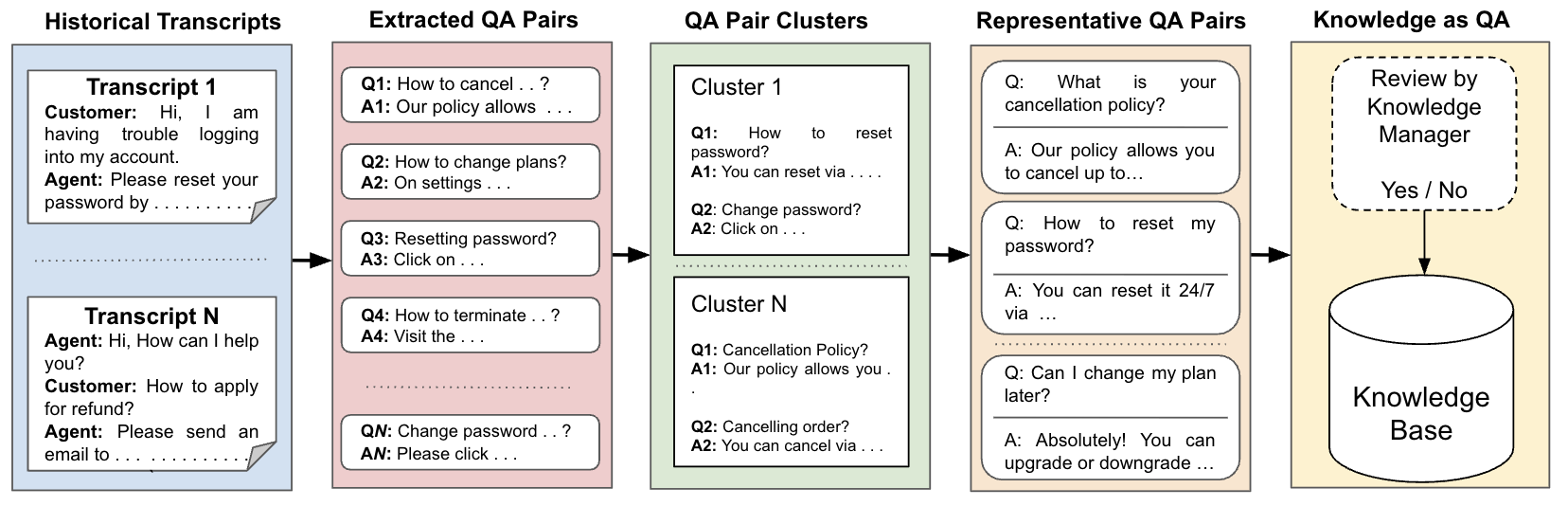
<p>The difference between Google and ChatGPT is that Google has to select good answers from external content in advance, while ChatGPT has to select good answers from responses generated internally.</p>

<p>Google’s blog post suggests three insights.</p>

<p><strong>First, Google must have invested substantial human-rater effort in evaluating search quality.</strong> The post discusses cases in which quality became a problem and shares a 182-page document called the <a href="https://static.googleusercontent.com/media/www.google.com/en//insidesearch/howsearchworks/assets/searchqualityevaluatorguidelines.pdf">Search Quality Rater Guidelines</a>. I expect that ChatGPT made a similar effort to ensure that Fast answers are trustworthy.</p>

<p><strong>Second, retrieval and the serving decision are separate problems.</strong> Storing and retrieving a good snippet is one problem; deciding whether to show it to the user is another. Google did not show a snippet when its authority, quality, or compatibility with the query was insufficient. Similarly, I will describe Fast answers as a three-stage system: curation, retrieval, and policy.</p>

<p><strong>Third, Google worked on cases in which queries were lexically similar but had different semantic intent.</strong> As mentioned above, its approach may have been to keep the number of snippets small to reduce management costs while solving the semantic query-matching problem. ChatGPT, however, provides internally generated content, which should make that content easier to generate and manage than Google’s external content. With that in mind, Fast answers may not have needed semantic query matching in its initial version.</p>

<h3 id="32-managing-qa-catalog">3.2 Managing QA Catalog</h3>

<p>While I could not find prior work that exactly matches the Fast answers setting, there is a substantial body of work on automatically building and maintaining FAQ-style knowledge bases from historical user interactions.<sup id="fnref:qa-catalog-literature"><a href="#fn:qa-catalog-literature" class="footnote" rel="footnote" role="doc-noteref">5</a></sup></p>

<p>The common idea is to mine recurring information needs from historical user queries or conversations, group semantically similar questions, and turn them into reusable question-answer pairs. These pairs can then form a prepared-answer catalog that a separate retrieval system may consult when a similar request arrives in the future.</p>

<p>One particularly relevant example is <a href="https://arxiv.org/abs/2510.08149">AI Knowledge Assist</a>. This paper follows the common approach described above and provides a concrete example of how such a system can be built.</p>

<p><img src="/assets/images/chatgpt-fast-answer-0/ai-knowledge-assist-overview.png" alt="Overview of the AI Knowledge Assist pipeline" />
<em>Figure 11. Overview of AI Knowledge Assist. Source: Figure 2 in <a href="https://aclanthology.org/2025.emnlp-industry.130/">Laskar et al. (2025)</a>, licensed under <a href="https://creativecommons.org/licenses/by/4.0/">CC BY 4.0</a>.</em></p>

<p>The paper assumes that many companies want to build conversational AI chatbots or RAG systems but do not have company-specific knowledge bases. However, if a company has customer service chat data, QA data is already embedded in the agents’ answers to customer questions. The paper therefore proposes a way to extract and clean this data and keep it updated over time. This is similar to ChatGPT’s situation: user chat logs already exist, and the task is to extract a QA set from them. However, the same question may have different answers in ChatGPT depending on each user’s context, so those answers cannot be used directly. The data could at least be used to identify recurring questions.</p>

<p>The paper uses LLMs in most stages. It first uses an LLM to extract reusable QA pairs from raw conversation data. Rather than extracting arbitrary pairs, it applies the following conditions: information-seeking, non-personalized, no PII, not time-sensitive, universal, and useful. It then clusters the QA pairs by question similarity and uses an LLM to select a representative QA pair from each cluster. A pair is either added automatically or sent for human review. The paper also mentions an automatic update mechanism that uses question similarity and answer similarity for future catalog updates.</p>

<p>In my view, there are three major points to consider when building a catalog system.</p>

<p><strong>First, QA pair filtering has to be done well.</strong> It effectively determines the final quality of the product. A clear policy is needed to define which kinds of questions align with the product’s goals. This is not something that can be solved simply by having a product owner write down a constitution-like set of rules. The initial policy will most likely contain many vague areas, creating conflicts no matter how closely a human rater or an LLM rater tries to follow it. The policy therefore has to improve through multiple iterations. A previous post from my time at Hyperconnect discusses this process in more detail.<sup id="fnref:policy-iteration"><a href="#fn:policy-iteration" class="footnote" rel="footnote" role="doc-noteref">6</a></sup></p>

<p><strong>Second, the decision to add a QA pair to the catalog will also likely be automated with an ML model, but designing that decision policy is not easy.</strong> For example, when setting a confidence cutoff, several variables have to be considered: whether the confidence comes from a calibrated model, how the cutoff affects human-rater costs, and how much total traffic the system receives. The problem is to find a Pareto-optimal point among these variables.</p>

<p><strong>Third, the system has to support continuous updates.</strong> Even seemingly stable catalogs can become stale over time, and the distribution of what counts as a good QA pair is likely to shift. The system should therefore be designed from the beginning to be robust to this shift. For example, as user-feedback data accumulates, the system should automatically adapt to distribution shifts so that its performance is maintained or improves over time.</p>

<h3 id="33-retrieval">3.3 Retrieval</h3>

<p>Once a good QA catalog has been built, the system has to retrieve the right entry for each user query. Although this system design assumes exact query matching to reduce system complexity, it is still worth identifying and comparing the other available options.</p>

<p>Information retrieval in modern ML systems is already a well-studied problem. Several papers have also explored it specifically in the FAQ retrieval domain.<sup id="fnref:faq-retrieval-literature"><a href="#fn:faq-retrieval-literature" class="footnote" rel="footnote" role="doc-noteref">7</a></sup> Each presents a novel idea, but the core modeling decisions come down to two questions:</p>

<ol>
  <li>How should relevance between a user query and a QA pair be defined?</li>
  <li>Should the retrieval target consider only the question, or the answer as well?</li>
</ol>

<p>As with any ML modeling problem, defining the objective is the most important step. For Fast answers, the retrieval objective could be aligned directly with the product objective: maximizing user satisfaction with the answer. However, user satisfaction can be sparse, noisy, and difficult to measure. In that case, an LLM-based prediction of user satisfaction could be used instead. An answerability score from a domain expert could also serve as a training proxy. Whatever signal is chosen, it should be quantifiable and aligned with the product objective, and the model should be trained to optimize it.</p>

<table class="comparison-table">
  <thead>
    <tr>
      <th>Query pair</th>
      <th>Answer</th>
      <th style="text-align: right">Cosine similarity</th>
    </tr>
  </thead>
  <tbody>
    <tr>
      <td><em>When was Python created?</em> ↔ <em>Who created Python?</em></td>
      <td><strong>1991 vs. Guido van Rossum</strong></td>
      <td style="text-align: right"><strong>0.927</strong></td>
    </tr>
    <tr>
      <td><em>Who created Python?</em> ↔ <em>Who was the original author of Python?</em></td>
      <td><strong>Both Guido van Rossum</strong></td>
      <td style="text-align: right"><strong>0.853</strong></td>
    </tr>
  </tbody>
</table>

<p><em>Table 1. Cosine similarities measured with <code class="language-plaintext highlighter-rouge">BAAI/bge-small-en-v1.5</code>.</em></p>

<p>The important point is that an off-the-shelf pretrained sentence embedding is unlikely to be aligned with the Fast answers objective. A general sentence embedding model considers the first query pair more similar than the second. However, the first pair requires different answers, while the second pair shares the same answer. Query similarity alone is therefore not necessarily aligned with answer equivalence. Fine-tuning for the actual objective is likely to be essential.</p>

<h3 id="34-final-decision-layer">3.4 Final Decision Layer</h3>

<p>So far, the discussion has focused on which QA pairs should be included in the candidate set and how to select the best one among them. A production-level system has to consider one more step: the decision policy that determines whether the selected QA pair should actually be shown to the user. In other words, the system has to answer this question automatically: <em>For this user, in this situation, is showing a Fast answer better than normal generation?</em> The need for this layer will be covered in the next system design post. For now, it is useful to examine how the QA domain has approached this problem.</p>

<p><em>vCache: Verified Semantic Prompt Caching</em><sup id="fnref:vcache"><a href="#fn:vcache" class="footnote" rel="footnote" role="doc-noteref">8</a></sup> is the paper most directly related to Fast answers. When a user query and a cached query are similar in embedding space, the cached response is reused. Rather than using one fixed similarity threshold, vCache assigns a separate threshold to each cached entry and learns those thresholds online to maximize cache hits while satisfying a user-specified global error-rate constraint. When the system is uncertain, it explores by invoking the underlying model, collects additional correctness observations, and uses them for online threshold learning. This is similar to the approach I would take for Fast answers. In my case, the objective would be to minimize LLM cost while maintaining user satisfaction rather than maximizing cache hits under a global error-rate constraint, and the technical details of learning the policy would also differ.</p>

<p><em>Selective Question Answering under Domain Shift</em><sup id="fnref:selective-qa"><a href="#fn:selective-qa" class="footnote" rel="footnote" role="doc-noteref">9</a></sup> uses gating to answer as many questions as possible while maintaining accuracy above a specified level. Its objective is therefore to maximize coverage subject to a target-accuracy constraint. Because naively using confidence can fail due to calibration problems, the paper trains a calibrator, a type of meta-model, and argues that it remains robust under domain shift. The objective is different, but the approach is similar in that it performs constrained optimization.</p>

<p><em>Generate-then-Retrieve: Intent-Aware FAQ Retrieval in Product Search</em><sup id="fnref:generate-then-retrieve-decision"><a href="#fn:generate-then-retrieve-decision" class="footnote" rel="footnote" role="doc-noteref">10</a></sup> takes the unusual approach of applying gating before retrieval. This is effective when a large amount of pruning can be done at the user-query level. Although the mechanism is different, exact matching in my design plays a similarly aggressive filtering role: only a narrow subset of queries is allowed to enter the Fast-answer path.</p>

<p>There are many possible decision policies. However, this layer can be made arbitrarily sophisticated, so the design here will keep only the essential pieces and focus on making the system extensible later. Whether a particular method matters should be tested and decided based on the product context. The more important point is to recognize the need for a decision layer and introduce the concept early in the product launch.</p>

<h2 id="4-from-observation-to-system-design">4. From Observation to System Design</h2>

<p>The rest of this series uses three working assumptions based on the product observations and related work discussed so far.</p>

<p>First, Fast answers are served from a catalog of pre-generated question-answer pairs rather than generated from scratch for every request. Second, to keep the initial system simple and minimize incorrect matches, I will assume that retrieval is based primarily on exact query matching. Third, retrieving a valid QA pair does not necessarily mean that it should be shown. A separate decision layer determines whether serving the Fast answer is preferable to normal LLM generation for a given user and context.</p>

<p>These assumptions are not claims about how ChatGPT is actually implemented. They are design choices I would make if I were responsible for launching the product. With this foundation in place, the next post moves from observation to system design.</p>

<hr />

<p>If you have read this far, something in this post probably caught your interest. If you would like to know more about me, feel free to <a href="https://www.linkedin.com/in/jjonghu">connect with me on LinkedIn</a>.</p>

<h2 id="references">References</h2>

<div class="footnotes" role="doc-endnotes">
  <ol>
    <li id="fn:release-note">
      <p>See the April 22, 2026 entry in the <a href="https://help.openai.com/en/articles/6825453-chatgpt-release-notes">ChatGPT release notes</a>. <a href="#fnref:release-note" class="reversefootnote" role="doc-backlink">&#8617;</a> <a href="#fnref:release-note:1" class="reversefootnote" role="doc-backlink">&#8617;<sup>2</sup></a></p>
    </li>
    <li id="fn:release-examples">
      <p>Repeated attempts did not trigger a Fast answer for either example. The football question requires fresh information, so it makes sense not to serve a ready-made answer. But why did the Seven Wonders question not trigger the feature? The answer was generated differently each time, while the same four images always appeared. This raises another question: does ChatGPT have a separate caching system for images? A later post will explore that possibility.</p>

      <div style="display: flex; gap: 0.5rem; align-items: flex-start;">
  <img src="/assets/images/chatgpt-fast-answer-0/wonder_0.png" alt="First generated response for Show me the Seven Wonders of the World" style="width: 50%;" />
  <img src="/assets/images/chatgpt-fast-answer-0/wonder_1.png" alt="Second generated response with the same images" style="width: 50%;" />
</div>
      <p><a href="#fnref:release-examples" class="reversefootnote" role="doc-backlink">&#8617;</a></p>
    </li>
    <li id="fn:korea-usage">
      <p>Korean has a relatively small global speaker base. However, supporting it may be a natural choice given how active South Korea is as a ChatGPT market: in June 2025, <a href="https://www.koreaherald.com/article/10500190">The Korea Herald reported that it ranked second globally in paid ChatGPT subscribers</a>, behind only the United States. <a href="#fnref:korea-usage" class="reversefootnote" role="doc-backlink">&#8617;</a></p>
    </li>
    <li id="fn:usage-paper">
      <p>See <a href="https://cdn.openai.com/pdf/a253471f-8260-40c6-a2cc-aa93fe9f142e/economic-research-chatgpt-usage-paper.pdf"><em>How People Use ChatGPT</em></a>, Figure 7 and Section 5.2. Seeking Information grew from 14% of messages in July 2024 to 24% in July 2025. <a href="#fnref:usage-paper" class="reversefootnote" role="doc-backlink">&#8617;</a></p>
    </li>
    <li id="fn:qa-catalog-literature">
      <p>Related work includes <a href="https://arxiv.org/abs/2510.08149"><em>AI Knowledge Assist: An Automated Approach for the Creation of Knowledge Bases for Conversational AI Agents</em></a> (2025); <a href="https://dl.acm.org/doi/10.1145/3731599.3767429"><em>Generating Frequently Asked Questions from Technical Support Tickets using Large Language Models</em></a> (2025); <a href="https://arxiv.org/abs/2601.04388"><em>LLM-Guided Lifecycle-Aware Clustering of Multi-Turn Customer Support Conversations</em></a> (2025); <a href="https://arxiv.org/abs/2212.07112"><em>DialogQAE: N-to-N Question Answer Pair Extraction from Customer Service Chatlog</em></a> (2023); and <a href="https://aclanthology.org/2023.acl-industry.22/"><em>Improving Knowledge Production Efficiency With Question Answering on Conversation</em></a> (2023). <a href="#fnref:qa-catalog-literature" class="reversefootnote" role="doc-backlink">&#8617;</a></p>
    </li>
    <li id="fn:policy-iteration">
      <p>See <a href="https://hyperconnect.github.io/2026/04/22/how-hyperconnect-built-llm-explanation-policy.html"><em>How Hyperconnect Built an LLM Explanation Policy</em></a>. The post is written in Korean, but I recommend reading it with translation. <a href="#fnref:policy-iteration" class="reversefootnote" role="doc-backlink">&#8617;</a></p>
    </li>
    <li id="fn:faq-retrieval-literature">
      <p>Related work includes <a href="https://aclanthology.org/2023.acl-industry.73/"><em>Generate-then-Retrieve: Intent-Aware FAQ Retrieval in Product Search</em></a> (2023); <a href="https://arxiv.org/abs/2304.01003"><em>QUADRo: Dataset and Models for Question-Answer Database Retrieval</em></a> (2023); <a href="https://aclanthology.org/2020.acl-main.74/"><em>Unsupervised FAQ Retrieval with Question Generation and BERT</em></a> (2020); and <a href="https://aclanthology.org/2024.eacl-short.41/"><em>Pre-Training Methods for Question Reranking</em></a> (2024). <a href="#fnref:faq-retrieval-literature" class="reversefootnote" role="doc-backlink">&#8617;</a></p>
    </li>
    <li id="fn:vcache">
      <p>See <a href="https://arxiv.org/abs/2502.03771"><em>vCache: Verified Semantic Prompt Caching</em></a>. <a href="#fnref:vcache" class="reversefootnote" role="doc-backlink">&#8617;</a></p>
    </li>
    <li id="fn:selective-qa">
      <p>See <a href="https://arxiv.org/abs/2006.09462"><em>Selective Question Answering under Domain Shift</em></a>. <a href="#fnref:selective-qa" class="reversefootnote" role="doc-backlink">&#8617;</a></p>
    </li>
    <li id="fn:generate-then-retrieve-decision">
      <p>See <a href="https://arxiv.org/abs/2306.03411"><em>Generate-then-Retrieve: Intent-Aware FAQ Retrieval in Product Search</em></a>. <a href="#fnref:generate-then-retrieve-decision" class="reversefootnote" role="doc-backlink">&#8617;</a></p>
    </li>
  </ol>
</div>]]></content><author><name>Jonghu</name></author><category term="system-design" /><category term="product" /><category term="literature-survey" /><category term="openai" /><summary type="html"><![CDATA[TL;DR ChatGPT has a feature called Fast answers.1 It appears to serve ready-made answers to frequently asked, information-seeking questions. What if I were the person responsible for launching it? For fun, I worked backward from the product and wrote a hypothetical system design. This is a four-part series. Part 0 covers my understanding of the product and a survey of the related literature. The rest of the system design continues in the following posts: Part 1. Business Context and ML System Design Part 2. Production Architecture Part 3. Operations and Continuous Improvement 1. ChatGPT Does Not Always Generate a New Response One day, I was solving a LeetCode problem and wanted to refresh my memory on quickselect. ChatGPT has become my go-to knowledge hub, so I naturally typed quickselect into it. This time, though, the answer came back surprisingly fast and was labeled Fast answer. Figure 1. My first encounter with a Fast answer in ChatGPT. It was the first time I had seen the feature, and I was curious enough to try the same query again. I opened another chat, typed quickselect, and got the same answer. That was unusual. An LLM will generally produce somewhat different responses even when it receives the same prompt twice. This time, the wording, structure, and examples were identical. My immediate guess was that ChatGPT was returning a stored query-answer pair instead of generating a fresh response. Query-answer caching would be a reasonable way to reduce both latency and inference cost for common questions with stable answers. That led me to a more interesting question: if I were building and launching this feature, how would I design it? What follows is a hypothetical design based on public information, a few product experiments, and assumptions I made myself. I have no inside knowledge of how Fast answers is actually implemented. 2. Product Observation A quick search did not reveal much, but the feature does appear in the ChatGPT release notes.1 Figure 2. OpenAI’s release note introducing Fast answers. The note says Fast answers are intended for common information-seeking questions, such as “Show me the Seven Wonders of the World” or “Which football team has the most Super Bowl titles?”2 ChatGPT may respond faster when two conditions hold: The question does not require a personalized response. ChatGPT has a high-confidence answer ready. It also says that Fast answers do not reference the user’s past chats or memory. The release note does not explain what “has a high-confidence answer ready” means technically. My working hypothesis is that ChatGPT maintains a collection of pre-generated answers for common, straightforward questions and returns one when an incoming query matches with sufficient confidence. That is the assumption I use throughout this series. A few small experiments helped clarify the product surface before considering the system behind it. These were informal observations rather than a controlled evaluation, and the behavior may change as the feature evolves. 2.1 The Same Query Returns the Same Answer Several frequently searched topics triggered Fast answers, including: quickselect why is the sky blue what is ROAS For these experiments, Fast answers were enabled under Settings → Personalization, with Intelligence set to Instant. With this setup, each query produced a Fast answer. Repeating a query in a new chat returned the same response. Figure 3. Fast answers for why is the sky blue and what is ROAS. Below a Fast answer, ChatGPT shows a lightning-bolt icon. Clicking it lets the user regenerate the answer immediately or describe in natural language how it should be regenerated. This button is probably one of the main channels for collecting user feedback. The system design later in this series will discuss how feedback from this surface could be used. Figure 4. The Fast answer menu offers regeneration and a free-form instruction field. 2.2 The Same Query Does Not Always Trigger It Even the exact same query did not always trigger a Fast answer. In the screenshot below, ChatGPT generated a response to quickselect and began answering in Korean. I normally use ChatGPT in Korean, so my memory or conversation history was probably included in the context for this response. Figure 5. The same quickselect query did not trigger a Fast answer this time. There are several possible reasons why the feature triggers inconsistently. OpenAI may still be running conversation-level A/B tests. There may be a heuristic that treats repeated submissions of the same query as dissatisfaction with the Fast answer and switches back to generation. Or some hidden logic may decide whether to show a Fast answer for each user based on personalized signals. This last possibility will be discussed in more detail in the system design. Regardless of the reason, randomized triggering may actually be the better launch strategy. Rather than always showing the cached result for the same query, it may be better to randomize whether the user receives the cached answer. The resulting data—including user reactions and inference-cost savings—could inform the next product decision. Randomized data would also reduce bias in later analysis and make counterfactual analysis more credible. The system design will cover this in more detail. 2.3 Semantically Similar Queries Return Different Answers At first, I thought the feature might use semantic search to retrieve answers for similar queries. For example, quickselect and what is quickselect can both be satisfied by a single answer explaining the concept. It would be reasonable to prepare one answer and return it for semantically similar user queries. Figure 6. quickselect and what is quickselect trigger different Fast answers. The actual behavior was different. As the screenshots show, even semantically equivalent queries returned different answers. This suggests that the current Fast answer system may store one answer per query and determine cache hits through exact query matching. There are two tradeoffs to consider: Maintain one polished answer, which makes answer-quality management easier, but requires solving semantic cache hit and miss decisions accurately. Use exact matching for queries, which keeps the lookup logic simple but increases the number of query-answer pairs to manage. From the perspective of launching and operating an initial system, the second approach may have been simpler. It makes sense if the product decision is that user disappointment from a false cache hit and a low-quality answer is more costly than the LLM generation cost of a false cache miss. The system design will examine this tradeoff in more detail. 2.4 It Appears to Support Multiple Languages The feature also triggered outside English, suggesting that eligibility is not limited to one language. As in Section 2.3, two questions with similar meanings received different answers. The screenshots below ask for the definition of ROAS using two different Korean expressions, and the responses are different as well. This supports the exact-query-matching hypothesis regardless of language. Figure 7. Two Korean queries asking for the definition of ROAS return different Fast answers. This was interesting because limiting an initial launch to English would normally be safer. Cached answers need to be reviewed for quality before they are served. Multilingual review adds outsourcing, coordination, and operational costs, so supporting a language with relatively few global speakers, such as Korean, would not be easy.3 This suggests two possibilities. First, OpenAI may believe that the cost savings from multilingual Fast answers are large enough to justify the additional review cost. Second, it may have enough confidence in an automated quality-review system to operate the feature across languages. 2.5 Fast Answers Have a Faster TTFT Browser developer tools showed a clear difference in how quickly the two response types began arriving. Using time to first response byte as a proxy for TTFT, Fast answers took roughly 400–600 ms, while normally generated answers took roughly 1.8–2.2 seconds. Figure 8. The Fast answer began arriving after about 559 ms. Figure 9. The normally generated answer began arriving after about 1.81 seconds. Interestingly, Fast answers were still delivered as a stream, even though the answers appeared to have been prepared in advance. These screenshots were taken in July 2026. When the feature first launched two months earlier, I remember the entire answer arriving more quickly without visible streaming. From a UX perspective, the response appeared to fill in immediately, which made the feature feel extremely fast. Something may have changed in the meantime. There are at least three possible explanations: The pre-generated-answer hypothesis is wrong, and Fast answers are actually generated by a very lightweight model. The answers are pre-generated, but OpenAI switched to streaming to keep the UX consistent with normal responses and may be A/B testing that presentation. The behavior changed for some other reason that cannot be observed from the outside. The goal of this series is not to reverse-engineer the feature exactly. It is to develop my own system design from the product behavior I can observe. I will therefore continue with the assumption that Fast answers return pre-generated responses. 2.6 It May Trigger in the Middle of a Conversation I expected this feature to apply only to the first query in a conversation. According to OpenAI’s study of how people use ChatGPT, 24% of messages were classified as Seeking Information as of July 2025—in other words, use that closely resembles search.4 Information-seeking traffic should contain frequently repeated queries, so I thought this feature was introduced to reduce LLM inference cost by caching answers to those queries. However, a comment in a Reddit discussion about Fast answers complains that a keyword triggered a Fast answer in the middle of a multi-turn conversation. In that case, ChatGPT ignored the context accumulated so far and returned an answer that had already been prepared. That behavior was unexpected. I do not know whether it is intended or a bug. In my design, I would probably allow Fast answers only for the first query. Once a conversation becomes multi-turn, the user is more likely to care about the context built up so far, which makes it much harder for a context-free Fast answer to satisfy them. 3. Related Products and Literature 3.1 Direct Answers Before LLMs Fast answers may look like a new LLM product feature, but search engines have long faced a similar problem. Google Featured Snippets extract an answer-like passage from a webpage and place it above the ordinary search results. Figure 10. A Google Featured Snippet answering the query “Why is the sky blue.” The difference between Google and ChatGPT is that Google has to select good answers from external content in advance, while ChatGPT has to select good answers from responses generated internally. Google’s blog post suggests three insights. First, Google must have invested substantial human-rater effort in evaluating search quality. The post discusses cases in which quality became a problem and shares a 182-page document called the Search Quality Rater Guidelines. I expect that ChatGPT made a similar effort to ensure that Fast answers are trustworthy. Second, retrieval and the serving decision are separate problems. Storing and retrieving a good snippet is one problem; deciding whether to show it to the user is another. Google did not show a snippet when its authority, quality, or compatibility with the query was insufficient. Similarly, I will describe Fast answers as a three-stage system: curation, retrieval, and policy. Third, Google worked on cases in which queries were lexically similar but had different semantic intent. As mentioned above, its approach may have been to keep the number of snippets small to reduce management costs while solving the semantic query-matching problem. ChatGPT, however, provides internally generated content, which should make that content easier to generate and manage than Google’s external content. With that in mind, Fast answers may not have needed semantic query matching in its initial version. 3.2 Managing QA Catalog While I could not find prior work that exactly matches the Fast answers setting, there is a substantial body of work on automatically building and maintaining FAQ-style knowledge bases from historical user interactions.5 The common idea is to mine recurring information needs from historical user queries or conversations, group semantically similar questions, and turn them into reusable question-answer pairs. These pairs can then form a prepared-answer catalog that a separate retrieval system may consult when a similar request arrives in the future. One particularly relevant example is AI Knowledge Assist. This paper follows the common approach described above and provides a concrete example of how such a system can be built. Figure 11. Overview of AI Knowledge Assist. Source: Figure 2 in Laskar et al. (2025), licensed under CC BY 4.0. The paper assumes that many companies want to build conversational AI chatbots or RAG systems but do not have company-specific knowledge bases. However, if a company has customer service chat data, QA data is already embedded in the agents’ answers to customer questions. The paper therefore proposes a way to extract and clean this data and keep it updated over time. This is similar to ChatGPT’s situation: user chat logs already exist, and the task is to extract a QA set from them. However, the same question may have different answers in ChatGPT depending on each user’s context, so those answers cannot be used directly. The data could at least be used to identify recurring questions. The paper uses LLMs in most stages. It first uses an LLM to extract reusable QA pairs from raw conversation data. Rather than extracting arbitrary pairs, it applies the following conditions: information-seeking, non-personalized, no PII, not time-sensitive, universal, and useful. It then clusters the QA pairs by question similarity and uses an LLM to select a representative QA pair from each cluster. A pair is either added automatically or sent for human review. The paper also mentions an automatic update mechanism that uses question similarity and answer similarity for future catalog updates. In my view, there are three major points to consider when building a catalog system. First, QA pair filtering has to be done well. It effectively determines the final quality of the product. A clear policy is needed to define which kinds of questions align with the product’s goals. This is not something that can be solved simply by having a product owner write down a constitution-like set of rules. The initial policy will most likely contain many vague areas, creating conflicts no matter how closely a human rater or an LLM rater tries to follow it. The policy therefore has to improve through multiple iterations. A previous post from my time at Hyperconnect discusses this process in more detail.6 Second, the decision to add a QA pair to the catalog will also likely be automated with an ML model, but designing that decision policy is not easy. For example, when setting a confidence cutoff, several variables have to be considered: whether the confidence comes from a calibrated model, how the cutoff affects human-rater costs, and how much total traffic the system receives. The problem is to find a Pareto-optimal point among these variables. Third, the system has to support continuous updates. Even seemingly stable catalogs can become stale over time, and the distribution of what counts as a good QA pair is likely to shift. The system should therefore be designed from the beginning to be robust to this shift. For example, as user-feedback data accumulates, the system should automatically adapt to distribution shifts so that its performance is maintained or improves over time. 3.3 Retrieval Once a good QA catalog has been built, the system has to retrieve the right entry for each user query. Although this system design assumes exact query matching to reduce system complexity, it is still worth identifying and comparing the other available options. Information retrieval in modern ML systems is already a well-studied problem. Several papers have also explored it specifically in the FAQ retrieval domain.7 Each presents a novel idea, but the core modeling decisions come down to two questions: How should relevance between a user query and a QA pair be defined? Should the retrieval target consider only the question, or the answer as well? As with any ML modeling problem, defining the objective is the most important step. For Fast answers, the retrieval objective could be aligned directly with the product objective: maximizing user satisfaction with the answer. However, user satisfaction can be sparse, noisy, and difficult to measure. In that case, an LLM-based prediction of user satisfaction could be used instead. An answerability score from a domain expert could also serve as a training proxy. Whatever signal is chosen, it should be quantifiable and aligned with the product objective, and the model should be trained to optimize it. Query pair Answer Cosine similarity When was Python created? ↔ Who created Python? 1991 vs. Guido van Rossum 0.927 Who created Python? ↔ Who was the original author of Python? Both Guido van Rossum 0.853 Table 1. Cosine similarities measured with BAAI/bge-small-en-v1.5. The important point is that an off-the-shelf pretrained sentence embedding is unlikely to be aligned with the Fast answers objective. A general sentence embedding model considers the first query pair more similar than the second. However, the first pair requires different answers, while the second pair shares the same answer. Query similarity alone is therefore not necessarily aligned with answer equivalence. Fine-tuning for the actual objective is likely to be essential. 3.4 Final Decision Layer So far, the discussion has focused on which QA pairs should be included in the candidate set and how to select the best one among them. A production-level system has to consider one more step: the decision policy that determines whether the selected QA pair should actually be shown to the user. In other words, the system has to answer this question automatically: For this user, in this situation, is showing a Fast answer better than normal generation? The need for this layer will be covered in the next system design post. For now, it is useful to examine how the QA domain has approached this problem. vCache: Verified Semantic Prompt Caching8 is the paper most directly related to Fast answers. When a user query and a cached query are similar in embedding space, the cached response is reused. Rather than using one fixed similarity threshold, vCache assigns a separate threshold to each cached entry and learns those thresholds online to maximize cache hits while satisfying a user-specified global error-rate constraint. When the system is uncertain, it explores by invoking the underlying model, collects additional correctness observations, and uses them for online threshold learning. This is similar to the approach I would take for Fast answers. In my case, the objective would be to minimize LLM cost while maintaining user satisfaction rather than maximizing cache hits under a global error-rate constraint, and the technical details of learning the policy would also differ. Selective Question Answering under Domain Shift9 uses gating to answer as many questions as possible while maintaining accuracy above a specified level. Its objective is therefore to maximize coverage subject to a target-accuracy constraint. Because naively using confidence can fail due to calibration problems, the paper trains a calibrator, a type of meta-model, and argues that it remains robust under domain shift. The objective is different, but the approach is similar in that it performs constrained optimization. Generate-then-Retrieve: Intent-Aware FAQ Retrieval in Product Search10 takes the unusual approach of applying gating before retrieval. This is effective when a large amount of pruning can be done at the user-query level. Although the mechanism is different, exact matching in my design plays a similarly aggressive filtering role: only a narrow subset of queries is allowed to enter the Fast-answer path. There are many possible decision policies. However, this layer can be made arbitrarily sophisticated, so the design here will keep only the essential pieces and focus on making the system extensible later. Whether a particular method matters should be tested and decided based on the product context. The more important point is to recognize the need for a decision layer and introduce the concept early in the product launch. 4. From Observation to System Design The rest of this series uses three working assumptions based on the product observations and related work discussed so far. First, Fast answers are served from a catalog of pre-generated question-answer pairs rather than generated from scratch for every request. Second, to keep the initial system simple and minimize incorrect matches, I will assume that retrieval is based primarily on exact query matching. Third, retrieving a valid QA pair does not necessarily mean that it should be shown. A separate decision layer determines whether serving the Fast answer is preferable to normal LLM generation for a given user and context. These assumptions are not claims about how ChatGPT is actually implemented. They are design choices I would make if I were responsible for launching the product. With this foundation in place, the next post moves from observation to system design. If you have read this far, something in this post probably caught your interest. If you would like to know more about me, feel free to connect with me on LinkedIn. References See the April 22, 2026 entry in the ChatGPT release notes. &#8617; &#8617;2 Repeated attempts did not trigger a Fast answer for either example. The football question requires fresh information, so it makes sense not to serve a ready-made answer. But why did the Seven Wonders question not trigger the feature? The answer was generated differently each time, while the same four images always appeared. This raises another question: does ChatGPT have a separate caching system for images? A later post will explore that possibility. &#8617; Korean has a relatively small global speaker base. However, supporting it may be a natural choice given how active South Korea is as a ChatGPT market: in June 2025, The Korea Herald reported that it ranked second globally in paid ChatGPT subscribers, behind only the United States. &#8617; See How People Use ChatGPT, Figure 7 and Section 5.2. Seeking Information grew from 14% of messages in July 2024 to 24% in July 2025. &#8617; Related work includes AI Knowledge Assist: An Automated Approach for the Creation of Knowledge Bases for Conversational AI Agents (2025); Generating Frequently Asked Questions from Technical Support Tickets using Large Language Models (2025); LLM-Guided Lifecycle-Aware Clustering of Multi-Turn Customer Support Conversations (2025); DialogQAE: N-to-N Question Answer Pair Extraction from Customer Service Chatlog (2023); and Improving Knowledge Production Efficiency With Question Answering on Conversation (2023). &#8617; See How Hyperconnect Built an LLM Explanation Policy. The post is written in Korean, but I recommend reading it with translation. &#8617; Related work includes Generate-then-Retrieve: Intent-Aware FAQ Retrieval in Product Search (2023); QUADRo: Dataset and Models for Question-Answer Database Retrieval (2023); Unsupervised FAQ Retrieval with Question Generation and BERT (2020); and Pre-Training Methods for Question Reranking (2024). &#8617; See vCache: Verified Semantic Prompt Caching. &#8617; See Selective Question Answering under Domain Shift. &#8617; See Generate-then-Retrieve: Intent-Aware FAQ Retrieval in Product Search. &#8617;]]></summary><media:thumbnail xmlns:media="http://search.yahoo.com/mrss/" url="https://jonghu.github.io/assets/default-social-image.png" /><media:content medium="image" url="https://jonghu.github.io/assets/default-social-image.png" xmlns:media="http://search.yahoo.com/mrss/" /></entry><entry><title type="html">LLM-as-a-Judge in Practice</title><link href="https://jonghu.github.io/posts/llm-as-a-judge-in-practice/" rel="alternate" type="text/html" title="LLM-as-a-Judge in Practice" /><published>2026-07-10T14:00:00-05:00</published><updated>2026-07-10T14:00:00-05:00</updated><id>https://jonghu.github.io/posts/llm-as-a-judge-in-practice</id><content type="html" xml:base="https://jonghu.github.io/posts/llm-as-a-judge-in-practice/"><![CDATA[<p>This post summarizes the principles I keep in mind whenever I use LLM-as-a-Judge to evaluate and improve a system. Most of them come from my experience building LLM Judges while working at Hyperconnect<sup id="fnref:hyperconnect-judge"><a href="#fn:hyperconnect-judge" class="footnote" rel="footnote" role="doc-noteref">1</a></sup> and from Hamel Husain’s writing.<sup id="fnref:hamel-judge-guide"><a href="#fn:hamel-judge-guide" class="footnote" rel="footnote" role="doc-noteref">2</a></sup></p>

<p>What I want to discuss here is not how to prompt an LLM Judge. It is how to treat an LLM Judge as an ML system component and <strong>build an evaluation loop that lets us continuously optimize a system in the direction we actually want</strong>.</p>

<h2 id="you-cant-improve-what-you-cant-measure">You Can’t Improve What You Can’t Measure</h2>

<p>It is a well-known saying. If we cannot measure which version of a system is better, we cannot know what to improve. On the other hand, if we can measure the direction we want with a reasonably quantitative signal, we can use that signal to train models, compare experiments, analyze failures, and continuously improve the system.</p>

<p>A similar idea comes up frequently in AI today: if a problem is verifiable, it can eventually be optimized through reinforcement learning or a related method.<sup id="fnref:verifiers-rule"><a href="#fn:verifiers-rule" class="footnote" rel="footnote" role="doc-noteref">3</a></sup> The reward does not have to be perfect. If we can produce a signal that is sufficiently related to the direction we want, we can begin an optimization loop.</p>

<p>For generative features or search results whose quality is difficult to evaluate programmatically, it is natural to consider LLM-as-a-Judge. For example, a chatbot team may want to evaluate the helpfulness, conciseness, or correctness of a response. A search team may want to measure query-document relevance. In the past, humans labeled these subjective qualities directly. Now, part of that work can be delegated to an LLM Judge.</p>

<p>But introducing an LLM Judge immediately requires caution. Just because an LLM Judge produces a number does not mean that increasing that number will produce the system we actually want. If we optimize the Judge score aggressively but the real user experience or business outcome does not improve at all, we have not optimized the system well. We may simply have optimized the wrong objective very efficiently.</p>

<p>Before building an LLM Judge, it is therefore worth taking one step back.</p>

<h2 id="do-you-really-need-an-llm-judge">Do You Really Need an LLM Judge?</h2>

<p>First, ask whether there are any programmatic or directly observable signals that can evaluate the quality you care about.</p>

<p>Consider approaches such as RLVR, or Reinforcement Learning with Verifiable Rewards. In coding tasks, we can programmatically verify whether the final answer is correct, whether the code runs, whether it passes tests, and whether it satisfies the required format.</p>

<p>These signals do not perfectly express every kind of code quality we care about. Passing tests does not necessarily mean that code is readable or maintainable. In other words, these signals are incomplete with respect to the quality we ultimately want. But they are still highly reliable for an important part of that quality.</p>

<p>To simplify the idea, let $U$ be the user utility we ultimately want to optimize and $M$ be a measurable proxy signal. We do not need:</p>

\[M = U\]

<p>In practice, finding such a perfect metric is difficult.</p>

<p>What matters instead is whether the following relationship generally holds:</p>

\[M \uparrow \quad \Rightarrow \quad U \text{ also tends to } \uparrow\]

<p>The first question is whether an imperfect signal is still useful enough to move the system in the right direction.</p>

<p>For a consumer product, when evaluation is difficult, a useful starting point is the business objective: what does the product ultimately need to accomplish? From there, work backward through the user journey or funnel to identify measurable signals.</p>

<p>Suppose we are building an AI chatbot for customer support. Its ultimate business objective might be:</p>

\[\begin{aligned}
\min \quad &amp;\text{Customer Support Cost} \\
\text{subject to} \quad &amp;\text{Customer Satisfaction} \geq C
\end{aligned}\]

<p>In other words, the goal is to reduce support costs while keeping customer satisfaction above an acceptable level.</p>

<p>What does reducing support costs mean in practice?</p>

<p>One proxy is whether the AI chatbot resolves the user’s problem before escalating it to a human agent. We can measure the escalation rate. But a lack of escalation does not necessarily mean the problem was resolved. The user may simply have given up.</p>

<p>We can also ask whether the user reported that the problem was resolved after the conversation. We might examine whether the user contacts support again about the same issue within a certain period, or whether the ticket is reopened.</p>

<p>The problem can be decomposed in the following direction:</p>

\[\begin{gathered}
\text{Business Objective}
\rightarrow \text{Product Outcome} \\
\rightarrow \text{User Behavior}
\rightarrow \text{Measurable Signal}
\end{gathered}\]

<p>Each signal is clearly noisy and suboptimal. But taken together, several signals may cover a substantial portion of the original objective.</p>

<p>Before building an LLM Judge, ask:</p>

<blockquote>
  <p>Can programmatic or directly observable signals already capture enough of the objective we want to achieve?</p>
</blockquote>

<p>If they can, those signals are the better starting point.</p>

<h2 id="its-hard-to-eval-is-a-product-smell">“It’s Hard to Eval” Is a Product Smell</h2>

<p>If, after all this, we still cannot find any way to evaluate whether the product is working, it is worth asking whether something else is wrong. To borrow Hamel Husain’s phrase, “It’s Hard to Eval” Is a Product Smell.<sup id="fnref:eval-smell"><a href="#fn:eval-smell" class="footnote" rel="footnote" role="doc-noteref">4</a></sup></p>

<p>If the goal of a product is to satisfy customers but there is no way at all to determine whether customers are satisfied, we may not have defined clearly enough what we are trying to satisfy.</p>

<p>Of course, some final business outcomes appear only after several months. Causal attribution can be difficult, and signals can be extremely sparse. This is not an argument that every product has a perfect and immediate metric.</p>

<p>But a product ultimately solves some problem for a user. There must be a process through which the user moves from having that problem to having it resolved. If we understand the product and the user’s problem well enough, we should be able to break that process into smaller steps or define intermediate outcomes that provide some way to check whether the system is moving in the right direction.</p>

<p>If even that is difficult, evaluation may not be the only problem. We may need to revisit whether the product objective is clear enough, or whether the product itself is designed so that the user’s problem-solving process can be observed and verified.</p>

<h2 id="so-when-should-you-use-an-llm-judge">So, When Should You Use an LLM Judge?</h2>

<p>After thinking through the questions above, we may find several quantitative signals but still feel that they are too noisy or fail to cover an important part of the product objective. That is when an LLM Judge becomes worth considering. An LLM Judge can also be useful before a product has launched, when real user signals are not yet available.</p>

<p>A problem is a good candidate for an LLM Judge when it satisfies roughly the following conditions.</p>

<ul>
  <li>Measuring this quality would help improve the system.</li>
  <li>The quality is subjective and difficult to calculate directly.</li>
  <li>A sufficiently trained human can still judge it relatively consistently.</li>
  <li>Repeating that judgment at scale would make it useful in a real optimization loop.</li>
</ul>

<p>Consider query-document relevance in search. Relevance is difficult to calculate through simple string overlap. But in most cases, a domain expert who reads both the query and the document can judge whether the document is relevant to the query. This is a good candidate for an LLM Judge.</p>

<p>An LLM Judge is not a tool for solving problems where even humans do not know what good looks like. It is more appropriate for:</p>

<blockquote>
  <p>Problems that humans can judge, but where human judgment is difficult to scale.</p>
</blockquote>

<h2 id="what-makes-a-good-judge">What Makes a Good Judge?</h2>

<p>What conditions should an LLM Judge satisfy once it has been built? There are at least three.</p>

<ul>
  <li>It must produce a quantifiable signal that can be used to compare systems and optimize them.</li>
  <li>It must agree sufficiently with the judgment of the human experts best qualified to assess that quality.</li>
  <li>Improving the resulting offline signal should move the real user signal or business outcome in the same direction.</li>
</ul>

<p>This reveals two separate alignment problems. The first is the alignment of the Judge itself:</p>

\[J(x) \approx H(x)\]

<p>Here, $J$ is the judgment produced by the LLM Judge and $H$ is the judgment of a human expert.</p>

<p>But this alone is not enough. Ultimately, we also need:</p>

\[H(x) \approx U(x)\]

<p>Here, $U$ is actual user utility or the product objective.</p>

<p>Even if an LLM Judge achieves 95% agreement with human experts, we may still be measuring the wrong objective very precisely if the human experts’ criteria are not aligned with real user outcomes.</p>

<p>It is therefore important to separate the following two relationships:</p>

\[\text{LLM Judge} \leftrightarrow \text{Human Expert}\]

<p>and:</p>

\[\text{Offline Evaluation} \leftrightarrow \text{Online Product Outcome}\]

<p>The first is a Judge-calibration problem. The second asks whether the evaluation objective itself is correct.</p>

<h2 id="align-humans-before-aligning-the-judge">Align Humans Before Aligning the Judge</h2>

<p>People are often less aligned on subjective problems than we expect. Before building an LLM Judge, it is therefore useful to align the humans first.</p>

<p>Collect enough real system outputs, then ask the relevant domain experts, PMs, or even MLEs to label them independently. It is important to record not only a simple Pass or Fail, but also the reasoning or critique behind each judgment.</p>

<p>When the results are compared, there will probably be more disagreement than expected at first. These disagreements are the most valuable samples. They identify the current <strong>gray decision boundary</strong> of the product.</p>

<p>Comparing critiques and discussing why the judgments differ reveals implicit assumptions that the existing rubric did not specify.</p>

\[\begin{gathered}
\text{Human Disagreement}
\rightarrow
\text{Discussion} \\
\rightarrow
\text{Implicit Assumption}
\rightarrow
\text{Rubric Update}
\end{gathered}\]

<p>The team can then evaluate the outputs again with the updated rubric. As this process repeats, disagreement gradually decreases and human judgments begin to converge.</p>

<p>Importantly, this process updates more than the rubric document. It also updates the team’s implicit understanding of the product. The decision boundary becomes clearer:</p>

<blockquote>
  <p>What counts as a good output for this product?</p>
</blockquote>

<blockquote>
  <p>What is still acceptable, and where does it become unacceptable?</p>
</blockquote>

<p>As a result, the team develops domain experts who can judge the relevant product quality with reasonable consistency.</p>

<p>There is also a useful side effect. Repeating this process naturally creates a human-labeled dataset.</p>

<h2 id="iterate-and-update-the-rubric">Iterate and Update the Rubric</h2>

<p>A rubric cannot be made perfect from the beginning. It is more natural for the rubric to emerge from real outputs and failures.</p>

<p>Evaluate outputs with the initial rubric, find disagreements, compare critiques, and update the rubric. Then evaluate new samples again.</p>

\[\begin{gathered}
R_0 \rightarrow \text{Label} \rightarrow \text{Disagreement} \\
\downarrow \\
R_1 \rightarrow \text{Label} \rightarrow \text{Disagreement} \\
\downarrow \\
R_2 \rightarrow \cdots
\end{gathered}\]

<p>After enough iterations, major changes to the rubric become less frequent and human agreement stabilizes. Only then can we say that “what our team considers a good output” has become reasonably explicit.</p>

<p>The dataset accumulated by this point can later serve as a calibration dataset for evaluating and improving the LLM Judge.</p>

<h2 id="make-evaluation-as-simple-as-possible">Make Evaluation as Simple as Possible</h2>

<p>To make human alignment easier, the evaluation itself should be kept as simple as possible.</p>

<p>When possible, binary evaluation is a useful starting point. Using a Likert scale from 1 to 5 requires answers to questions such as:</p>

<blockquote>
  <p>What exactly is the difference between a 3 and a 4?</p>
</blockquote>

<blockquote>
  <p>Is a 4 good enough to ship to production?</p>
</blockquote>

<blockquote>
  <p>If one person gives the same output a 3 and another gives it a 4, is that truly a disagreement?</p>
</blockquote>

<p>Defining the meaning of every tick becomes another difficult problem.</p>

<p>Binary evaluation, in contrast, focuses on a single decision boundary:</p>

<blockquote>
  <p>Does this output satisfy the standard we want?</p>
</blockquote>

<p>Or, in more product-oriented language:</p>

<blockquote>
  <p>Would you ship this output?</p>
</blockquote>

<p>Even if each sample is evaluated in binary terms, aggregating those decisions produces a quantitative metric:</p>

\[\text{Pass Rate}
=
\frac{\#\text{Pass}}{\#\text{Total Samples}}\]

<p>This metric can compare model A with model B or detect regressions.</p>

<p>Of course, binary evaluation compresses a great deal of information. The tradeoff can be framed this way:</p>

<ul>
  <li>Binary for optimization</li>
  <li>Critiques for diagnosis</li>
</ul>

<p>Pass or Fail supports quantitative comparison and optimization. Detailed critiques explain why the system failed and help identify the next improvement.</p>

<h2 id="treat-the-judge-as-a-model-not-an-oracle">Treat the Judge as a Model, Not an Oracle</h2>

<p>Once the rubric has stabilized and a human-labeled dataset exists, we can build the LLM Judge.</p>

<p>A reasonable starting point is to place the rubric in the prompt and provide examples and critiques written by human experts as few-shot examples.</p>

<p>But the important point is not to trust the LLM Judge as an oracle. The Judge is still a model. We can represent the human-labeled dataset as:</p>

\[D_H = \{(x_i, y_i, c_i)\}_{i=1}^{N}\]

<p>Here, $x_i$ is the output being evaluated, $y_i$ is the human Pass or Fail label, and $c_i$ is the human critique.</p>

<p>For the same input, the LLM Judge produces:</p>

\[J(x_i) = (\hat{y}_i, \hat{c}_i)\]

<p>We can begin by comparing:</p>

\[\hat{y}_i \stackrel{?}{=} y_i\]

<p>This measures agreement between the Judge and the human.</p>

<p>But aggregate agreement is not enough. We need to inspect the samples that humans labeled Fail but the Judge labeled Pass, as well as those that humans labeled Pass but the Judge labeled Fail. Then we compare the Judge’s reasoning with the human critique. Analyzing these disagreements reveals where the Judge misunderstood the rubric, missed a condition, or lacked sufficient examples.</p>

<p>The interesting part is that this process has almost the same structure as the one above. First, we analyzed disagreements between:</p>

\[\text{Human} \leftrightarrow \text{Human}\]

<p>to improve the rubric.</p>

<p>Now, we analyze disagreements between:</p>

\[\text{Human} \leftrightarrow \text{Judge}\]

<p>to improve the prompt and the Judge.</p>

<p>In short:</p>

<blockquote>
  <p>Human-human disagreement $\rightarrow$ rubric iteration</p>
</blockquote>

<blockquote>
  <p>Human-Judge disagreement $\rightarrow$ Judge iteration</p>
</blockquote>

<p>By repeating this process, the Judge can gradually align with the decision boundary the team has established.</p>

<h2 id="optimize-the-system">Optimize the System</h2>

<p>Only now are we ready to use the offline evaluation signal produced by the LLM Judge to improve the actual system. We might change the model, improve the retrieval system, or modify the training data.</p>

<p>Each time, we use the same evaluation set and Judge to compare the previous system with the new one.</p>

\[S_0
\rightarrow
\text{Change}
\rightarrow
S_1
\rightarrow
\text{Offline Eval}\]

<p>If the Judge score improves, we move to the next iteration.</p>

<p>In this way, the LLM Judge is not merely a tool that evaluates whether a model is good. It becomes a measurement component inside the system-optimization loop.</p>

<h2 id="close-the-loop-with-online-evaluation">Close the Loop with Online Evaluation</h2>

<p>But the process cannot end there. As discussed earlier, alignment between the LLM Judge and human experts does not guarantee that the signal is aligned with actual user utility.</p>

<p>Once the system is deployed and user signals become available, we need to examine the relationship between offline evaluation and online outcomes.</p>

\[\begin{gathered}
\text{Offline Eval} \rightarrow \text{System Optimization} \\
\rightarrow \text{Deployment} \rightarrow \text{Online Evaluation}
\end{gathered}\]

<p>Then we ask the most important question:</p>

\[\text{Offline Eval} \uparrow
\quad \stackrel{?}{\Longrightarrow} \quad
\text{Online Outcome} \uparrow\]

<ul>
  <li>Did the model we judged to be better offline actually improve user satisfaction?</li>
  <li>When the search-relevance Judge improved, did engagement or task success improve as well?</li>
  <li>When the chatbot-resolution Judge improved, did the real escalation rate or repeat-contact rate improve?</li>
</ul>

<p>If not, improving the Judge itself may not be the priority. We need to return to the beginning and revisit whether the business objective, proxy signals, and human rubric were defined correctly. Then, if necessary, we start the iteration again.</p>

<h2 id="iterate-fast">Iterate Fast</h2>

<p>Finally, all of these iterations should happen quickly and frequently.  Do not try to create a perfect objective, a perfect rubric, or a perfect Judge from the start. This is such a familiar principle that I will not spend more time explaining it here.</p>

<h2 id="closing-the-loop">Closing the Loop</h2>

<p>Ultimately, when I use LLM-as-a-Judge, the Judge itself is not the most important part.</p>

<p>First, understand the business and the product, and define what we are ultimately trying to optimize.</p>

<p>Next, find measurable signals that serve as useful proxies for that objective. Prefer programmatic or directly observable signals when they are available.</p>

<p>If those signals cannot capture an important quality, and the remaining quality is subjective but trained humans can judge it relatively consistently, then consider an LLM Judge.</p>

<p>Before building the Judge, align the humans. Use human disagreements to discover the decision boundary and improve the rubric. Use the resulting human-labeled dataset to align the Judge with the humans.</p>

<p>Then use the Judge’s offline evaluation signal to optimize the system.</p>

<p>Finally, once the system meets real users, verify that the offline signal is aligned with the online product outcome.</p>

\[\boxed{
\begin{gathered}
\text{Business Objective}
\rightarrow
\text{Measurable Signals}
\rightarrow
\text{Human Alignment} \\
\rightarrow
\text{LLM Judge Alignment}
\rightarrow
\text{System Optimization} \\
\rightarrow
\text{Online Validation}
\rightarrow
\text{Repeat}
\end{gathered}
}\]

<p>To me, LLM-as-a-Judge is less a tool that scores outputs instead of a human and more an ML system component that makes part of an otherwise subjective and difficult-to-optimize product objective measurable.</p>

<p>Only when we continue iterating while checking that this measurement remains aligned with the direction we actually want can an LLM Judge play a meaningful role in continuously improving a system.</p>

<hr />

<p>If you have read this far, something in this post probably caught your interest. If you would like to know more about me, feel free to <a href="https://www.linkedin.com/in/jjonghu">connect with me on LinkedIn</a>.</p>

<h2 id="references">References</h2>

<div class="footnotes" role="doc-endnotes">
  <ol>
    <li id="fn:hyperconnect-judge">
      <p><a href="https://hyperconnect.github.io/2026/04/22/how-hyperconnect-built-llm-explanation-policy.html"><em>Part 1: No Data, No Ground Truth: How Hyperconnect Tamed an LLM</em></a> and <a href="https://hyperconnect.github.io/2026/04/22/llm-as-a-judge-for-explanation-quality.html"><em>Part 2: A Policy-Following Evaluator: LLM-as-a-Judge</em></a>. Both posts are written in Korean, but I recommend reading them with translation. <a href="#fnref:hyperconnect-judge" class="reversefootnote" role="doc-backlink">&#8617;</a></p>
    </li>
    <li id="fn:hamel-judge-guide">
      <p>Hamel Husain, <a href="https://hamel.dev/blog/posts/llm-judge/"><em>Using LLM-as-a-Judge for Evaluation: A Complete Guide</em></a>. His evaluation framework has been a major source of inspiration for me. <a href="#fnref:hamel-judge-guide" class="reversefootnote" role="doc-backlink">&#8617;</a></p>
    </li>
    <li id="fn:verifiers-rule">
      <p>Jason Wei, <a href="https://www.jasonwei.net/blog/asymmetry-of-verification-and-verifiers-law"><em>Asymmetry of Verification and Verifier’s Rule</em></a>. <a href="#fnref:verifiers-rule" class="reversefootnote" role="doc-backlink">&#8617;</a></p>
    </li>
    <li id="fn:eval-smell">
      <p>Hamel Husain, <a href="https://hamel.dev/blog/posts/eval-smell/"><em>“It’s Hard to Eval” Is a Product Smell</em></a>. His point is slightly different from the one I emphasize here: <strong>if developers find it difficult to evaluate the quality of an output, actual users are also likely to find it difficult to determine whether that output is correct</strong>. I borrowed the phrase because I agree with the underlying concern. <a href="#fnref:eval-smell" class="reversefootnote" role="doc-backlink">&#8617;</a></p>
    </li>
  </ol>
</div>]]></content><author><name>Jonghu</name></author><category term="evaluation" /><summary type="html"><![CDATA[This post summarizes the principles I keep in mind whenever I use LLM-as-a-Judge to evaluate and improve a system. Most of them come from my experience building LLM Judges while working at Hyperconnect1 and from Hamel Husain’s writing.2 What I want to discuss here is not how to prompt an LLM Judge. It is how to treat an LLM Judge as an ML system component and build an evaluation loop that lets us continuously optimize a system in the direction we actually want. You Can’t Improve What You Can’t Measure It is a well-known saying. If we cannot measure which version of a system is better, we cannot know what to improve. On the other hand, if we can measure the direction we want with a reasonably quantitative signal, we can use that signal to train models, compare experiments, analyze failures, and continuously improve the system. A similar idea comes up frequently in AI today: if a problem is verifiable, it can eventually be optimized through reinforcement learning or a related method.3 The reward does not have to be perfect. If we can produce a signal that is sufficiently related to the direction we want, we can begin an optimization loop. For generative features or search results whose quality is difficult to evaluate programmatically, it is natural to consider LLM-as-a-Judge. For example, a chatbot team may want to evaluate the helpfulness, conciseness, or correctness of a response. A search team may want to measure query-document relevance. In the past, humans labeled these subjective qualities directly. Now, part of that work can be delegated to an LLM Judge. But introducing an LLM Judge immediately requires caution. Just because an LLM Judge produces a number does not mean that increasing that number will produce the system we actually want. If we optimize the Judge score aggressively but the real user experience or business outcome does not improve at all, we have not optimized the system well. We may simply have optimized the wrong objective very efficiently. Before building an LLM Judge, it is therefore worth taking one step back. Do You Really Need an LLM Judge? First, ask whether there are any programmatic or directly observable signals that can evaluate the quality you care about. Consider approaches such as RLVR, or Reinforcement Learning with Verifiable Rewards. In coding tasks, we can programmatically verify whether the final answer is correct, whether the code runs, whether it passes tests, and whether it satisfies the required format. These signals do not perfectly express every kind of code quality we care about. Passing tests does not necessarily mean that code is readable or maintainable. In other words, these signals are incomplete with respect to the quality we ultimately want. But they are still highly reliable for an important part of that quality. To simplify the idea, let $U$ be the user utility we ultimately want to optimize and $M$ be a measurable proxy signal. We do not need: \[M = U\] In practice, finding such a perfect metric is difficult. What matters instead is whether the following relationship generally holds: \[M \uparrow \quad \Rightarrow \quad U \text{ also tends to } \uparrow\] The first question is whether an imperfect signal is still useful enough to move the system in the right direction. For a consumer product, when evaluation is difficult, a useful starting point is the business objective: what does the product ultimately need to accomplish? From there, work backward through the user journey or funnel to identify measurable signals. Suppose we are building an AI chatbot for customer support. Its ultimate business objective might be: \[\begin{aligned} \min \quad &amp;\text{Customer Support Cost} \\ \text{subject to} \quad &amp;\text{Customer Satisfaction} \geq C \end{aligned}\] In other words, the goal is to reduce support costs while keeping customer satisfaction above an acceptable level. What does reducing support costs mean in practice? One proxy is whether the AI chatbot resolves the user’s problem before escalating it to a human agent. We can measure the escalation rate. But a lack of escalation does not necessarily mean the problem was resolved. The user may simply have given up. We can also ask whether the user reported that the problem was resolved after the conversation. We might examine whether the user contacts support again about the same issue within a certain period, or whether the ticket is reopened. The problem can be decomposed in the following direction: \[\begin{gathered} \text{Business Objective} \rightarrow \text{Product Outcome} \\ \rightarrow \text{User Behavior} \rightarrow \text{Measurable Signal} \end{gathered}\] Each signal is clearly noisy and suboptimal. But taken together, several signals may cover a substantial portion of the original objective. Before building an LLM Judge, ask: Can programmatic or directly observable signals already capture enough of the objective we want to achieve? If they can, those signals are the better starting point. “It’s Hard to Eval” Is a Product Smell If, after all this, we still cannot find any way to evaluate whether the product is working, it is worth asking whether something else is wrong. To borrow Hamel Husain’s phrase, “It’s Hard to Eval” Is a Product Smell.4 If the goal of a product is to satisfy customers but there is no way at all to determine whether customers are satisfied, we may not have defined clearly enough what we are trying to satisfy. Of course, some final business outcomes appear only after several months. Causal attribution can be difficult, and signals can be extremely sparse. This is not an argument that every product has a perfect and immediate metric. But a product ultimately solves some problem for a user. There must be a process through which the user moves from having that problem to having it resolved. If we understand the product and the user’s problem well enough, we should be able to break that process into smaller steps or define intermediate outcomes that provide some way to check whether the system is moving in the right direction. If even that is difficult, evaluation may not be the only problem. We may need to revisit whether the product objective is clear enough, or whether the product itself is designed so that the user’s problem-solving process can be observed and verified. So, When Should You Use an LLM Judge? After thinking through the questions above, we may find several quantitative signals but still feel that they are too noisy or fail to cover an important part of the product objective. That is when an LLM Judge becomes worth considering. An LLM Judge can also be useful before a product has launched, when real user signals are not yet available. A problem is a good candidate for an LLM Judge when it satisfies roughly the following conditions. Measuring this quality would help improve the system. The quality is subjective and difficult to calculate directly. A sufficiently trained human can still judge it relatively consistently. Repeating that judgment at scale would make it useful in a real optimization loop. Consider query-document relevance in search. Relevance is difficult to calculate through simple string overlap. But in most cases, a domain expert who reads both the query and the document can judge whether the document is relevant to the query. This is a good candidate for an LLM Judge. An LLM Judge is not a tool for solving problems where even humans do not know what good looks like. It is more appropriate for: Problems that humans can judge, but where human judgment is difficult to scale. What Makes a Good Judge? What conditions should an LLM Judge satisfy once it has been built? There are at least three. It must produce a quantifiable signal that can be used to compare systems and optimize them. It must agree sufficiently with the judgment of the human experts best qualified to assess that quality. Improving the resulting offline signal should move the real user signal or business outcome in the same direction. This reveals two separate alignment problems. The first is the alignment of the Judge itself: \[J(x) \approx H(x)\] Here, $J$ is the judgment produced by the LLM Judge and $H$ is the judgment of a human expert. But this alone is not enough. Ultimately, we also need: \[H(x) \approx U(x)\] Here, $U$ is actual user utility or the product objective. Even if an LLM Judge achieves 95% agreement with human experts, we may still be measuring the wrong objective very precisely if the human experts’ criteria are not aligned with real user outcomes. It is therefore important to separate the following two relationships: \[\text{LLM Judge} \leftrightarrow \text{Human Expert}\] and: \[\text{Offline Evaluation} \leftrightarrow \text{Online Product Outcome}\] The first is a Judge-calibration problem. The second asks whether the evaluation objective itself is correct. Align Humans Before Aligning the Judge People are often less aligned on subjective problems than we expect. Before building an LLM Judge, it is therefore useful to align the humans first. Collect enough real system outputs, then ask the relevant domain experts, PMs, or even MLEs to label them independently. It is important to record not only a simple Pass or Fail, but also the reasoning or critique behind each judgment. When the results are compared, there will probably be more disagreement than expected at first. These disagreements are the most valuable samples. They identify the current gray decision boundary of the product. Comparing critiques and discussing why the judgments differ reveals implicit assumptions that the existing rubric did not specify. \[\begin{gathered} \text{Human Disagreement} \rightarrow \text{Discussion} \\ \rightarrow \text{Implicit Assumption} \rightarrow \text{Rubric Update} \end{gathered}\] The team can then evaluate the outputs again with the updated rubric. As this process repeats, disagreement gradually decreases and human judgments begin to converge. Importantly, this process updates more than the rubric document. It also updates the team’s implicit understanding of the product. The decision boundary becomes clearer: What counts as a good output for this product? What is still acceptable, and where does it become unacceptable? As a result, the team develops domain experts who can judge the relevant product quality with reasonable consistency. There is also a useful side effect. Repeating this process naturally creates a human-labeled dataset. Iterate and Update the Rubric A rubric cannot be made perfect from the beginning. It is more natural for the rubric to emerge from real outputs and failures. Evaluate outputs with the initial rubric, find disagreements, compare critiques, and update the rubric. Then evaluate new samples again. \[\begin{gathered} R_0 \rightarrow \text{Label} \rightarrow \text{Disagreement} \\ \downarrow \\ R_1 \rightarrow \text{Label} \rightarrow \text{Disagreement} \\ \downarrow \\ R_2 \rightarrow \cdots \end{gathered}\] After enough iterations, major changes to the rubric become less frequent and human agreement stabilizes. Only then can we say that “what our team considers a good output” has become reasonably explicit. The dataset accumulated by this point can later serve as a calibration dataset for evaluating and improving the LLM Judge. Make Evaluation as Simple as Possible To make human alignment easier, the evaluation itself should be kept as simple as possible. When possible, binary evaluation is a useful starting point. Using a Likert scale from 1 to 5 requires answers to questions such as: What exactly is the difference between a 3 and a 4? Is a 4 good enough to ship to production? If one person gives the same output a 3 and another gives it a 4, is that truly a disagreement? Defining the meaning of every tick becomes another difficult problem. Binary evaluation, in contrast, focuses on a single decision boundary: Does this output satisfy the standard we want? Or, in more product-oriented language: Would you ship this output? Even if each sample is evaluated in binary terms, aggregating those decisions produces a quantitative metric: \[\text{Pass Rate} = \frac{\#\text{Pass}}{\#\text{Total Samples}}\] This metric can compare model A with model B or detect regressions. Of course, binary evaluation compresses a great deal of information. The tradeoff can be framed this way: Binary for optimization Critiques for diagnosis Pass or Fail supports quantitative comparison and optimization. Detailed critiques explain why the system failed and help identify the next improvement. Treat the Judge as a Model, Not an Oracle Once the rubric has stabilized and a human-labeled dataset exists, we can build the LLM Judge. A reasonable starting point is to place the rubric in the prompt and provide examples and critiques written by human experts as few-shot examples. But the important point is not to trust the LLM Judge as an oracle. The Judge is still a model. We can represent the human-labeled dataset as: \[D_H = \{(x_i, y_i, c_i)\}_{i=1}^{N}\] Here, $x_i$ is the output being evaluated, $y_i$ is the human Pass or Fail label, and $c_i$ is the human critique. For the same input, the LLM Judge produces: \[J(x_i) = (\hat{y}_i, \hat{c}_i)\] We can begin by comparing: \[\hat{y}_i \stackrel{?}{=} y_i\] This measures agreement between the Judge and the human. But aggregate agreement is not enough. We need to inspect the samples that humans labeled Fail but the Judge labeled Pass, as well as those that humans labeled Pass but the Judge labeled Fail. Then we compare the Judge’s reasoning with the human critique. Analyzing these disagreements reveals where the Judge misunderstood the rubric, missed a condition, or lacked sufficient examples. The interesting part is that this process has almost the same structure as the one above. First, we analyzed disagreements between: \[\text{Human} \leftrightarrow \text{Human}\] to improve the rubric. Now, we analyze disagreements between: \[\text{Human} \leftrightarrow \text{Judge}\] to improve the prompt and the Judge. In short: Human-human disagreement $\rightarrow$ rubric iteration Human-Judge disagreement $\rightarrow$ Judge iteration By repeating this process, the Judge can gradually align with the decision boundary the team has established. Optimize the System Only now are we ready to use the offline evaluation signal produced by the LLM Judge to improve the actual system. We might change the model, improve the retrieval system, or modify the training data. Each time, we use the same evaluation set and Judge to compare the previous system with the new one. \[S_0 \rightarrow \text{Change} \rightarrow S_1 \rightarrow \text{Offline Eval}\] If the Judge score improves, we move to the next iteration. In this way, the LLM Judge is not merely a tool that evaluates whether a model is good. It becomes a measurement component inside the system-optimization loop. Close the Loop with Online Evaluation But the process cannot end there. As discussed earlier, alignment between the LLM Judge and human experts does not guarantee that the signal is aligned with actual user utility. Once the system is deployed and user signals become available, we need to examine the relationship between offline evaluation and online outcomes. \[\begin{gathered} \text{Offline Eval} \rightarrow \text{System Optimization} \\ \rightarrow \text{Deployment} \rightarrow \text{Online Evaluation} \end{gathered}\] Then we ask the most important question: \[\text{Offline Eval} \uparrow \quad \stackrel{?}{\Longrightarrow} \quad \text{Online Outcome} \uparrow\] Did the model we judged to be better offline actually improve user satisfaction? When the search-relevance Judge improved, did engagement or task success improve as well? When the chatbot-resolution Judge improved, did the real escalation rate or repeat-contact rate improve? If not, improving the Judge itself may not be the priority. We need to return to the beginning and revisit whether the business objective, proxy signals, and human rubric were defined correctly. Then, if necessary, we start the iteration again. Iterate Fast Finally, all of these iterations should happen quickly and frequently. Do not try to create a perfect objective, a perfect rubric, or a perfect Judge from the start. This is such a familiar principle that I will not spend more time explaining it here. Closing the Loop Ultimately, when I use LLM-as-a-Judge, the Judge itself is not the most important part. First, understand the business and the product, and define what we are ultimately trying to optimize. Next, find measurable signals that serve as useful proxies for that objective. Prefer programmatic or directly observable signals when they are available. If those signals cannot capture an important quality, and the remaining quality is subjective but trained humans can judge it relatively consistently, then consider an LLM Judge. Before building the Judge, align the humans. Use human disagreements to discover the decision boundary and improve the rubric. Use the resulting human-labeled dataset to align the Judge with the humans. Then use the Judge’s offline evaluation signal to optimize the system. Finally, once the system meets real users, verify that the offline signal is aligned with the online product outcome. \[\boxed{ \begin{gathered} \text{Business Objective} \rightarrow \text{Measurable Signals} \rightarrow \text{Human Alignment} \\ \rightarrow \text{LLM Judge Alignment} \rightarrow \text{System Optimization} \\ \rightarrow \text{Online Validation} \rightarrow \text{Repeat} \end{gathered} }\] To me, LLM-as-a-Judge is less a tool that scores outputs instead of a human and more an ML system component that makes part of an otherwise subjective and difficult-to-optimize product objective measurable. Only when we continue iterating while checking that this measurement remains aligned with the direction we actually want can an LLM Judge play a meaningful role in continuously improving a system. If you have read this far, something in this post probably caught your interest. If you would like to know more about me, feel free to connect with me on LinkedIn. References Part 1: No Data, No Ground Truth: How Hyperconnect Tamed an LLM and Part 2: A Policy-Following Evaluator: LLM-as-a-Judge. Both posts are written in Korean, but I recommend reading them with translation. &#8617; Hamel Husain, Using LLM-as-a-Judge for Evaluation: A Complete Guide. His evaluation framework has been a major source of inspiration for me. &#8617; Jason Wei, Asymmetry of Verification and Verifier’s Rule. &#8617; Hamel Husain, “It’s Hard to Eval” Is a Product Smell. His point is slightly different from the one I emphasize here: if developers find it difficult to evaluate the quality of an output, actual users are also likely to find it difficult to determine whether that output is correct. I borrowed the phrase because I agree with the underlying concern. &#8617;]]></summary><media:thumbnail xmlns:media="http://search.yahoo.com/mrss/" url="https://jonghu.github.io/assets/default-social-image.png" /><media:content medium="image" url="https://jonghu.github.io/assets/default-social-image.png" xmlns:media="http://search.yahoo.com/mrss/" /></entry><entry><title type="html">Building a Data Preprocessing Agent</title><link href="https://jonghu.github.io/posts/data-agent/" rel="alternate" type="text/html" title="Building a Data Preprocessing Agent" /><published>2026-05-25T22:22:47-05:00</published><updated>2026-05-25T22:22:47-05:00</updated><id>https://jonghu.github.io/posts/data-agent</id><content type="html" xml:base="https://jonghu.github.io/posts/data-agent/"><![CDATA[<h2 id="tldr">TL;DR</h2>

<ul>
  <li>I built a data preprocessing agent with my teammates <a href="https://www.linkedin.com/in/hsien-hao-li/">Max</a>, <a href="https://www.linkedin.com/in/sean-kraemer/">Sean</a>, and <a href="https://www.linkedin.com/in/shreya-rao-98903524b">Shreya</a>.</li>
  <li>We built a benchmark suite called <a href="/posts/kagglebench/">KaggleBench</a>. The novel idea is to evaluate agents on high-quality, human-expert data preprocessing workflows selected from Kaggle, rather than synthetic data.</li>
  <li>We built an agent with a workflow and tools tailored specifically to this task. We also built the agentic loop from scratch to understand the internals of AI agents.</li>
  <li>It was fun!</li>
</ul>

<p>You can take a look at the details of the <a href="/assets/reports/CS498_TEAM8_Project_Final_Benchmark_Paper.pdf">benchmark</a> and the <a href="/assets/reports/CS498_TEAM8_Project_Final_Agent_Paper.pdf">agent</a>!</p>

<h2 id="how-it-started">How it started</h2>

<p>In CS 498 AI Agents in the Wild, we worked on a project where we designed both an AI agent and a benchmark from scratch.</p>

<p>We spent the most time choosing the topic. Since we were going to spend a semester on it, we wanted the result to be meaningful. Even though this was a student project funded out of pocket, we wanted the outcome to be high quality enough to be proud of.</p>

<p>So we made decisions using three rules.</p>

<ol>
  <li>The topic should only be solvable with an agentic system. If a rule-based system or traditional machine learning could solve the problem well enough, we should avoid it.</li>
  <li>The topic should be measurable and quantifiable. We needed a dataset and a metric that could be justified reasonably. This matters because we wanted to show that our system works better than a simple baseline or prior work, and more importantly, that we can evaluate the system in a way that makes sense. If we cannot measure progress, we cannot improve the system in a disciplined way.<sup id="fnref:measurement"><a href="#fn:measurement" class="footnote" rel="footnote" role="doc-noteref">1</a></sup></li>
  <li>It should be possible to frame the topic as a problem with real industrial interest. The topic itself did not have to be industry-specific, but the core idea had to matter in industry. A research assistant agent maps naturally to information retrieval and summarization from user queries. A multi-turn customer service agent maps to chatting under policy constraints while retrieving information. These patterns are useful to many companies.</li>
</ol>

<p>After comparing several ideas by pros, cons, feasibility, and viability, we decided to study whether an agent can solve data preprocessing tasks. The topic fit our rules. First, it is essentially a coding problem, so it is hard to solve without an agent. Second, by using Kaggle, we thought we could turn it into a quasi-quantifiable evaluation problem. Third, data science agents are already a visible industrial use case. OpenAI has written about its internal data agent, and Databricks also documents a data science agent workflow in notebooks.<sup id="fnref:openai-data-agent"><a href="#fn:openai-data-agent" class="footnote" rel="footnote" role="doc-noteref">2</a></sup><sup id="fnref:databricks-ds-agent"><a href="#fn:databricks-ds-agent" class="footnote" rel="footnote" role="doc-noteref">3</a></sup></p>

<p>That is how we started working on the problem.</p>

<h2 id="kagglebench">KaggleBench</h2>

<p>For any system, defining quantitative evaluation first is important. Many LLM-based features or agent projects end with qualitative demos. The generated text looks impressive, and the project stops at subjective impressions. That is fun, but it does not create a path for improvement. Without a measurement setup, it is hard to know whether the next version is actually better.</p>

<p>At first glance, data preprocessing sounds like a small subset of a data science agent. But if you think about it carefully, it is not that different from a coding or math-solving problem. A data science project starts from ambiguous context, an imperfectly specified objective, and an open-ended search space. There is often no single perfect answer. Given how much money is being invested into coding agents, it would be unrealistic for a student team to solve the fully open-ended version in one semester.</p>

<p>So we had to scope the problem down. We reframed it as a multiple-choice decision problem. Given a Kaggle competition, its dataset, a set of candidate preprocessing actions, and a set of actions already taken, the agent has to decide which action should be added or removed.</p>

<p>This framing makes evaluation much easier because the problem is no longer fully open-ended. The hard part becomes generating good candidate actions. A good candidate action has to be clearly right or clearly wrong. It should not depend too much on subjective judgment.</p>

<p>For that, we used human-expert Kaggle notebooks as the source of truth. The details of how we built the dataset and evaluation suite are in the <a href="/posts/kagglebench/">KaggleBench post</a>.</p>

<h2 id="data-preprocessing-agent-from-scratch">Data preprocessing agent from scratch</h2>

<p>One constraint from the class was that we could not use a well-known agent SDK such as LangGraph. That was a useful constraint. At a high level, an agent can sound simple. You call an LLM in a loop, parse tool calls, execute tools, and feed the result back into the next step.</p>

<p>The real difficulty is not the loop itself. The important parts are the harness around it and the durable execution behavior. The agent needs the right tools, the right prompt structure, the right state representation, and a way to keep making progress without losing track of the task.</p>

<p>There are already many emerging practices around agent harness design. We selected a few that fit our setting and built the architecture around them. We also implemented the agentic loop ourselves so that we could understand what is happening inside the system instead of treating an SDK as a black box.</p>

<p>We evaluated the agent against several baselines, including rule-based heuristics and a naive agentic loop. The baselines were designed so that our final method could be understood as a combination of smaller design choices. That made the comparison work like an ablation study. We also compared against Claude Code to see how our task-specific agent performed against a commercial general-purpose coding agent.</p>

<p>The detailed implementation and results are in the <a href="/posts/data-agent-arch/">agent architecture post</a>.</p>

<h2 id="what-i-learned">What I Learned</h2>

<p>I got two main things from this project.</p>

<p>First, I learned a lot about agent architecture. Building an agent from scratch gave me a clearer big-picture understanding and more confidence. Of course, what we built was still an application-layer system that combined existing components. Each layer hides a lot of depth. Frontier labs know how to train LLMs with reinforcement learning for agentic use cases. LLM API providers do serious engineering around caching and request orchestration to use GPU resources efficiently. Agent harnesses for long-running tasks need many layers of reliability engineering. This project gave me a practical taste of what has to be considered at the application layer to build an end product.</p>

<p>Second, I got much better at using agents. Codex played a huge role in the development process. Because of it, I could spend more time on planning and decisions, which raised the quality of the final project. But it was not enough to simply hand off requests. I had to check persistently whether the thing I wanted had actually happened. That check could not only be conversational. I needed mechanical checks, tests, or direct inspection of outputs.</p>

<p>That process helped me feel the limitations of coding agents in a way that metrics alone cannot show. It was also interesting to experience model improvements during the project, from Codex 5.3 to 5.5.</p>

<h2 id="reference">Reference</h2>

<div class="footnotes" role="doc-endnotes">
  <ol>
    <li id="fn:measurement">
      <p>Commonly attributed to Peter Drucker. <a href="#fnref:measurement" class="reversefootnote" role="doc-backlink">&#8617;</a></p>
    </li>
    <li id="fn:openai-data-agent">
      <p><a href="https://openai.com/index/inside-our-in-house-data-agent/">Inside OpenAI’s in-house data agent</a> <a href="#fnref:openai-data-agent" class="reversefootnote" role="doc-backlink">&#8617;</a></p>
    </li>
    <li id="fn:databricks-ds-agent">
      <p><a href="https://docs.databricks.com/aws/en/notebooks/ds-agent">Databricks, Use Genie Code for data science</a> <a href="#fnref:databricks-ds-agent" class="reversefootnote" role="doc-backlink">&#8617;</a></p>
    </li>
  </ol>
</div>]]></content><author><name>Jonghu</name></author><category term="side-project" /><summary type="html"><![CDATA[TL;DR I built a data preprocessing agent with my teammates Max, Sean, and Shreya. We built a benchmark suite called KaggleBench. The novel idea is to evaluate agents on high-quality, human-expert data preprocessing workflows selected from Kaggle, rather than synthetic data. We built an agent with a workflow and tools tailored specifically to this task. We also built the agentic loop from scratch to understand the internals of AI agents. It was fun! You can take a look at the details of the benchmark and the agent! How it started In CS 498 AI Agents in the Wild, we worked on a project where we designed both an AI agent and a benchmark from scratch. We spent the most time choosing the topic. Since we were going to spend a semester on it, we wanted the result to be meaningful. Even though this was a student project funded out of pocket, we wanted the outcome to be high quality enough to be proud of. So we made decisions using three rules. The topic should only be solvable with an agentic system. If a rule-based system or traditional machine learning could solve the problem well enough, we should avoid it. The topic should be measurable and quantifiable. We needed a dataset and a metric that could be justified reasonably. This matters because we wanted to show that our system works better than a simple baseline or prior work, and more importantly, that we can evaluate the system in a way that makes sense. If we cannot measure progress, we cannot improve the system in a disciplined way.1 It should be possible to frame the topic as a problem with real industrial interest. The topic itself did not have to be industry-specific, but the core idea had to matter in industry. A research assistant agent maps naturally to information retrieval and summarization from user queries. A multi-turn customer service agent maps to chatting under policy constraints while retrieving information. These patterns are useful to many companies. After comparing several ideas by pros, cons, feasibility, and viability, we decided to study whether an agent can solve data preprocessing tasks. The topic fit our rules. First, it is essentially a coding problem, so it is hard to solve without an agent. Second, by using Kaggle, we thought we could turn it into a quasi-quantifiable evaluation problem. Third, data science agents are already a visible industrial use case. OpenAI has written about its internal data agent, and Databricks also documents a data science agent workflow in notebooks.23 That is how we started working on the problem. KaggleBench For any system, defining quantitative evaluation first is important. Many LLM-based features or agent projects end with qualitative demos. The generated text looks impressive, and the project stops at subjective impressions. That is fun, but it does not create a path for improvement. Without a measurement setup, it is hard to know whether the next version is actually better. At first glance, data preprocessing sounds like a small subset of a data science agent. But if you think about it carefully, it is not that different from a coding or math-solving problem. A data science project starts from ambiguous context, an imperfectly specified objective, and an open-ended search space. There is often no single perfect answer. Given how much money is being invested into coding agents, it would be unrealistic for a student team to solve the fully open-ended version in one semester. So we had to scope the problem down. We reframed it as a multiple-choice decision problem. Given a Kaggle competition, its dataset, a set of candidate preprocessing actions, and a set of actions already taken, the agent has to decide which action should be added or removed. This framing makes evaluation much easier because the problem is no longer fully open-ended. The hard part becomes generating good candidate actions. A good candidate action has to be clearly right or clearly wrong. It should not depend too much on subjective judgment. For that, we used human-expert Kaggle notebooks as the source of truth. The details of how we built the dataset and evaluation suite are in the KaggleBench post. Data preprocessing agent from scratch One constraint from the class was that we could not use a well-known agent SDK such as LangGraph. That was a useful constraint. At a high level, an agent can sound simple. You call an LLM in a loop, parse tool calls, execute tools, and feed the result back into the next step. The real difficulty is not the loop itself. The important parts are the harness around it and the durable execution behavior. The agent needs the right tools, the right prompt structure, the right state representation, and a way to keep making progress without losing track of the task. There are already many emerging practices around agent harness design. We selected a few that fit our setting and built the architecture around them. We also implemented the agentic loop ourselves so that we could understand what is happening inside the system instead of treating an SDK as a black box. We evaluated the agent against several baselines, including rule-based heuristics and a naive agentic loop. The baselines were designed so that our final method could be understood as a combination of smaller design choices. That made the comparison work like an ablation study. We also compared against Claude Code to see how our task-specific agent performed against a commercial general-purpose coding agent. The detailed implementation and results are in the agent architecture post. What I Learned I got two main things from this project. First, I learned a lot about agent architecture. Building an agent from scratch gave me a clearer big-picture understanding and more confidence. Of course, what we built was still an application-layer system that combined existing components. Each layer hides a lot of depth. Frontier labs know how to train LLMs with reinforcement learning for agentic use cases. LLM API providers do serious engineering around caching and request orchestration to use GPU resources efficiently. Agent harnesses for long-running tasks need many layers of reliability engineering. This project gave me a practical taste of what has to be considered at the application layer to build an end product. Second, I got much better at using agents. Codex played a huge role in the development process. Because of it, I could spend more time on planning and decisions, which raised the quality of the final project. But it was not enough to simply hand off requests. I had to check persistently whether the thing I wanted had actually happened. That check could not only be conversational. I needed mechanical checks, tests, or direct inspection of outputs. That process helped me feel the limitations of coding agents in a way that metrics alone cannot show. It was also interesting to experience model improvements during the project, from Codex 5.3 to 5.5. Reference Commonly attributed to Peter Drucker. &#8617; Inside OpenAI’s in-house data agent &#8617; Databricks, Use Genie Code for data science &#8617;]]></summary><media:thumbnail xmlns:media="http://search.yahoo.com/mrss/" url="https://jonghu.github.io/assets/default-social-image.png" /><media:content medium="image" url="https://jonghu.github.io/assets/default-social-image.png" xmlns:media="http://search.yahoo.com/mrss/" /></entry><entry><title type="html">KaggleBench</title><link href="https://jonghu.github.io/posts/kagglebench/" rel="alternate" type="text/html" title="KaggleBench" /><published>2026-05-25T22:21:47-05:00</published><updated>2026-05-25T22:21:47-05:00</updated><id>https://jonghu.github.io/posts/kagglebench</id><content type="html" xml:base="https://jonghu.github.io/posts/kagglebench/"><![CDATA[<h2 id="tldr">TL;DR</h2>

<p>Coming soon… You can take a look at the details of the <a href="/assets/reports/CS498_TEAM8_Project_Final_Benchmark_Paper.pdf">benchmark</a> and the <a href="/assets/reports/CS498_TEAM8_Project_Final_Agent_Paper.pdf">agent</a>!</p>]]></content><author><name>Jonghu</name></author><category term="evaluation" /><summary type="html"><![CDATA[TL;DR Coming soon… You can take a look at the details of the benchmark and the agent!]]></summary><media:thumbnail xmlns:media="http://search.yahoo.com/mrss/" url="https://jonghu.github.io/assets/default-social-image.png" /><media:content medium="image" url="https://jonghu.github.io/assets/default-social-image.png" xmlns:media="http://search.yahoo.com/mrss/" /></entry><entry><title type="html">Data Agent Architecture</title><link href="https://jonghu.github.io/posts/data-agent-arch/" rel="alternate" type="text/html" title="Data Agent Architecture" /><published>2026-05-25T22:20:47-05:00</published><updated>2026-05-25T22:20:47-05:00</updated><id>https://jonghu.github.io/posts/data-agent-arch</id><content type="html" xml:base="https://jonghu.github.io/posts/data-agent-arch/"><![CDATA[<h2 id="tldr">TL;DR</h2>]]></content><author><name>Jonghu</name></author><category term="agent" /><summary type="html"><![CDATA[TL;DR]]></summary><media:thumbnail xmlns:media="http://search.yahoo.com/mrss/" url="https://jonghu.github.io/assets/default-social-image.png" /><media:content medium="image" url="https://jonghu.github.io/assets/default-social-image.png" xmlns:media="http://search.yahoo.com/mrss/" /></entry><entry><title type="html">Hacker News Data Pipeline</title><link href="https://jonghu.github.io/posts/hn-data-pipeline/" rel="alternate" type="text/html" title="Hacker News Data Pipeline" /><published>2026-05-24T20:28:28-05:00</published><updated>2026-05-24T20:28:28-05:00</updated><id>https://jonghu.github.io/posts/hn-data-pipeline</id><content type="html" xml:base="https://jonghu.github.io/posts/hn-data-pipeline/"><![CDATA[<h2 id="tldr">TL;DR</h2>

<ul>
  <li>I built a data pipeline that stores public events from Hacker News.</li>
  <li>The first goal was data analysis, but I also wanted a reusable event backbone for future HN projects, including recommendation systems.</li>
  <li>Tech Stack: EC2, SQS, Lambda, DynamoDB, Kinesis Data Firehose, S3, Athena, CloudWatch, Terraform, and Docker.</li>
</ul>

<p>The data collected by this pipeline was used in <a href="/posts/hn-analysis/">When Does a Post Go Viral on Hacker News?</a>.</p>

<h2 id="why-i-built-this">Why I Built This</h2>

<p>Hacker News already has a public API.<sup id="fnref:hn-api"><a href="#fn:hn-api" class="footnote" rel="footnote" role="doc-noteref">1</a></sup> It exposes a useful view of the current HN ecosystem, including item details, user profiles, recently changed items and profiles, and the current Top Stories list.</p>

<p>That is enough for many applications. If I want to show the current title, score, and comments for a story, the API is fine. For the analysis I had in mind, though, the current state was not enough. I was interested in the dynamics of the system. I wanted to know what path a post took before it reached the Top 10, how its upvotes accumulated, when comments arrived, when it moved between pages, and whether author-level signals were useful later.</p>

<p>Those questions need snapshots over time. A final item record does not tell me how the item got there.</p>

<p>So I decided to build my own pipeline. Part of the motivation was practical. I needed the data for analysis. I also wanted to practice building something closer to a real data pipeline than a local scraper.</p>

<p>For Hacker News scale, the simplest system might have been one EC2 instance that polls the API and writes files directly to disk or S3. That probably would have been cheaper and easier. I intentionally chose a more overbuilt design because I wanted to practice the shape of a larger production data system. That meant queues, serverless workers, latest-state storage, append-only archives, CDC, monitoring, and infrastructure-as-code.</p>

<p>That made the project more complicated than it strictly needed to be. The extra complexity gave me a reusable base for later HN work. Once I have item snapshots, ranking events, and user snapshots in a consistent format, I can attach other pipelines on top for causal analysis, recommender experiments, author features, topic modeling, or personalized ranking.</p>

<h2 id="hacker-news-api-overview">Hacker News API Overview</h2>

<p>The HN API is small, but it has the pieces needed to observe the public surface of the site.</p>

<p>The first entity is an item. In HN, stories, comments, jobs, polls, and poll options are all items. They live under this endpoint.</p>

<div class="language-text highlighter-rouge"><div class="highlight"><pre class="highlight"><code>/v0/item/&lt;id&gt;.json
</code></pre></div></div>

<p>An item can have fields like <code class="language-plaintext highlighter-rouge">id</code>, <code class="language-plaintext highlighter-rouge">type</code>, <code class="language-plaintext highlighter-rouge">by</code>, <code class="language-plaintext highlighter-rouge">time</code>, <code class="language-plaintext highlighter-rouge">title</code>, <code class="language-plaintext highlighter-rouge">url</code>, <code class="language-plaintext highlighter-rouge">text</code>, <code class="language-plaintext highlighter-rouge">score</code>, <code class="language-plaintext highlighter-rouge">kids</code>, <code class="language-plaintext highlighter-rouge">descendants</code>, <code class="language-plaintext highlighter-rouge">dead</code>, and <code class="language-plaintext highlighter-rouge">deleted</code>. This is the main entity for the item pipeline.</p>

<p>The second entity is a user.</p>

<div class="language-text highlighter-rouge"><div class="highlight"><pre class="highlight"><code>/v0/user/&lt;id&gt;.json
</code></pre></div></div>

<p>A user record contains fields like <code class="language-plaintext highlighter-rouge">id</code>, <code class="language-plaintext highlighter-rouge">created</code>, <code class="language-plaintext highlighter-rouge">karma</code>, <code class="language-plaintext highlighter-rouge">about</code>, and <code class="language-plaintext highlighter-rouge">submitted</code>. I used this for author context and future recommender features.</p>

<p>The API also exposes live-ish change surfaces.</p>

<div class="language-text highlighter-rouge"><div class="highlight"><pre class="highlight"><code>/v0/updates.json
/v0/topstories.json
</code></pre></div></div>

<p><code class="language-plaintext highlighter-rouge">updates.json</code> returns recently changed item IDs and profile IDs. I used it as the source for the item and user pipelines. <code class="language-plaintext highlighter-rouge">topstories.json</code> returns the current Top Stories ranking list, up to 500 items. I used it to build ranking snapshots and ranking events.</p>

<h2 id="item-pipeline">Item Pipeline</h2>

<p><img src="/assets/images/hn-data-pipeline/pipeline_item.png" alt="Item pipeline architecture" /></p>

<p><em>Figure 1. Item pipeline from HN updates to raw snapshots and derived change events.</em></p>

<p>The item pipeline is the main pipeline.</p>

<p>It starts with an EC2 poller. The poller reads <code class="language-plaintext highlighter-rouge">updates.json</code>, looks at the <code class="language-plaintext highlighter-rouge">items</code> array, and detects item IDs that were not in the previous poll. It sends those IDs to SQS.</p>

<p>The next step is a Lambda fetcher. The fetcher reads item IDs from SQS, calls <code class="language-plaintext highlighter-rouge">/v0/item/&lt;id&gt;.json</code>, computes a deterministic hash of the HN payload, and writes the latest item state to DynamoDB only if the payload changed. When it writes a changed item, it also sends the raw item snapshot to Firehose, which writes compressed JSONL files into S3.</p>

<p>DynamoDB Streams are enabled on the latest-items table. A second Lambda receives old and new images from the stream, compares the <code class="language-plaintext highlighter-rouge">item</code> field, and emits field-level change events to another Firehose stream. Those events also land in S3.</p>

<p>So the item pipeline has two S3 outputs.</p>

<div class="language-text highlighter-rouge"><div class="highlight"><pre class="highlight"><code>raw item snapshots
item change events
</code></pre></div></div>

<p>This split was deliberate. The raw snapshot is the safer source of truth. The event stream is a derived convenience layer. If I later decide that an event definition was wrong, I can recompute it from raw snapshots.</p>

<p>The advantage of this design is that each piece has a simple job. The poller detects changes. SQS absorbs bursts. Lambda fetches item details. DynamoDB holds the latest state. S3 holds history. The CDC Lambda turns state changes into analysis-friendly events.</p>

<p>The downside is obvious. This is more moving parts than HN strictly requires. It also has a small blind spot around poller restarts because the poller keeps its previous baseline in memory. If the poller restarts, it takes a fresh baseline and only catches later diffs. I accepted this because the goal was not perfect archival of every possible API state. I wanted a reliable enough public-event history for analysis.</p>

<h2 id="top-stories-pipeline">Top Stories Pipeline</h2>

<p><img src="/assets/images/hn-data-pipeline/pipeline_top.png" alt="Top Stories pipeline architecture" /></p>

<p><em>Figure 2. Top Stories pipeline for rank snapshots and rank movement events.</em></p>

<p>The Top Stories pipeline tracks visibility.</p>

<p>The HN item API tells me an item’s score and metadata, but it does not tell me when the item was on page 1, when it crossed from rank 31 to rank 30, or how long it stayed near the top. For that, I needed ranking snapshots.</p>

<p>The top stories poller reads <code class="language-plaintext highlighter-rouge">topstories.json</code> on a fixed interval. For each snapshot, it writes the ranked list to Firehose and S3. It also compares the current ranking with the previous ranking and emits rank events.</p>

<div class="language-text highlighter-rouge"><div class="highlight"><pre class="highlight"><code>APPEAR
DISAPPEAR
RANK_UP
RANK_DOWN
</code></pre></div></div>

<p>The advantage is that ranking dynamics become explicit. I can ask when an item first appeared in Top Stories, whether it reached the Top 30, how long it stayed visible, and how rank movement related to later upvotes.</p>

<p>The tradeoff is storage volume. A full ranking snapshot writes many records even when the ranking only changes a little. In this pipeline, that tradeoff was acceptable because the records are simple, compressed S3 storage is cheap, and the analysis becomes much easier. I would rather store a slightly redundant ranking history than reconstruct visibility from partial state later.</p>

<h2 id="user-pipeline">User Pipeline</h2>

<p><img src="/assets/images/hn-data-pipeline/pipeline_user.png" alt="User pipeline architecture" /></p>

<p><em>Figure 3. User pipeline for profile snapshots and historical author backfill.</em></p>

<p>The user pipeline came later and had the lowest priority.</p>

<p>Conceptually, it is similar to the item pipeline. A user poller reads the <code class="language-plaintext highlighter-rouge">profiles</code> field from <code class="language-plaintext highlighter-rouge">updates.json</code> and sends changed user IDs to SQS. A Lambda fetcher calls <code class="language-plaintext highlighter-rouge">/v0/user/&lt;id&gt;.json</code>, stores the latest user profile in DynamoDB, and archives raw snapshots to S3 through Firehose.</p>

<p>The main difference is that I did not build a CDC event pipeline for users.</p>

<p>User records have much less dynamic structure than items. For my use case, I mostly needed author context such as karma, account age, profile text, and submitted history. Field-level user events were not important enough to justify another stream.</p>

<p>The biggest operational decision was user backfill. Since the user pipeline was added after the item pipeline, I needed a backfill to recover author profiles for historical items. I used a residual backfill instead of a blind one to avoid redundant HN API calls for users already collected by the live pipeline. I started with small canaries, then 100 users, then 1,000, then 5,000, and eventually continued in 5,000-user chunks. The rate ceiling stayed at 5 users per second. The pace was conservative. It kept the live queue healthy and avoided unnecessary load on HN.</p>

<h2 id="observability-and-operation">Observability and Operation</h2>

<p>The operational goal was not to build a perfect monitoring system. I wanted enough observability to know whether the pipeline was alive, whether queues were backing up, and whether data was still reaching S3.</p>

<p>The pollers publish CloudWatch metrics such as heartbeat, poll latency, and number of enqueued IDs. SQS queue age is the main downstream health signal. If the poller heartbeat is present while the queue age is rising, the fetcher side is not keeping up.</p>

<p>I also added a small monitoring layer with CloudWatch alarms, SNS email alerts, and a weekly summary Lambda. The summary checks monitored surfaces, throughput, alarm history, queue health, and coarse S3 freshness. It can tell me that the monitored surfaces look healthy, but it cannot prove every individual record was processed exactly as intended. That was the right level for a small always-on research pipeline.</p>

<p>Infrastructure was deployed with Terraform where I wanted a repeatable control plane. The pollers ran as Docker containers under systemd on EC2. Lambda deployment used scripts and packaged zip artifacts. S3 data was queried with Athena when I needed quick checks or lightweight analysis. I also added small cost controls later, including batched CloudWatch metric publication, lower heartbeat frequency, and log retention.</p>

<h2 id="results-and-takeaway">Results and Takeaway</h2>

<p>The archive contains item data from November 17, 2025 UTC through May 11, 2026 UTC. The Top Stories archive starts on November 27, 2025 UTC. The user archive starts on March 18, 2026 UTC.</p>

<p>Across that period, CloudWatch and S3 show roughly the following volume.</p>

<ul>
  <li>9.4M raw item snapshot records sent to Firehose</li>
  <li>10.6M item change event records sent to Firehose</li>
  <li>218.2M Top Stories rank snapshot records sent to Firehose</li>
  <li>29.0M Top Stories rank event records sent to Firehose</li>
  <li>2.7M raw user snapshot records sent to Firehose</li>
  <li>26.0M item SQS messages received</li>
  <li>2.8M user SQS messages received</li>
</ul>

<p>Operationally, I would not claim literal zero errors. CloudWatch shows a small number of transient Lambda errors across millions of invocations. I did not see a sustained pipeline incident in the metrics I checked. Firehose failed-put metrics were zero, and max queue age stayed bounded during the archived period.</p>

<p>I think this was partly because the system was not actually very complex. HN is also a stable community site rather than a high-variance traffic source. The traffic is large enough to be interesting and small enough that a conservative AWS pipeline can handle it comfortably.</p>

<h2 id="references">References</h2>

<div class="footnotes" role="doc-endnotes">
  <ol>
    <li id="fn:hn-api">
      <p><a href="https://github.com/HackerNews/API">HackerNews/API, documentation and samples for the official HN API</a> <a href="#fnref:hn-api" class="reversefootnote" role="doc-backlink">&#8617;</a></p>
    </li>
  </ol>
</div>]]></content><author><name>Jonghu</name></author><category term="data" /><summary type="html"><![CDATA[TL;DR I built a data pipeline that stores public events from Hacker News. The first goal was data analysis, but I also wanted a reusable event backbone for future HN projects, including recommendation systems. Tech Stack: EC2, SQS, Lambda, DynamoDB, Kinesis Data Firehose, S3, Athena, CloudWatch, Terraform, and Docker. The data collected by this pipeline was used in When Does a Post Go Viral on Hacker News?. Why I Built This Hacker News already has a public API.1 It exposes a useful view of the current HN ecosystem, including item details, user profiles, recently changed items and profiles, and the current Top Stories list. That is enough for many applications. If I want to show the current title, score, and comments for a story, the API is fine. For the analysis I had in mind, though, the current state was not enough. I was interested in the dynamics of the system. I wanted to know what path a post took before it reached the Top 10, how its upvotes accumulated, when comments arrived, when it moved between pages, and whether author-level signals were useful later. Those questions need snapshots over time. A final item record does not tell me how the item got there. So I decided to build my own pipeline. Part of the motivation was practical. I needed the data for analysis. I also wanted to practice building something closer to a real data pipeline than a local scraper. For Hacker News scale, the simplest system might have been one EC2 instance that polls the API and writes files directly to disk or S3. That probably would have been cheaper and easier. I intentionally chose a more overbuilt design because I wanted to practice the shape of a larger production data system. That meant queues, serverless workers, latest-state storage, append-only archives, CDC, monitoring, and infrastructure-as-code. That made the project more complicated than it strictly needed to be. The extra complexity gave me a reusable base for later HN work. Once I have item snapshots, ranking events, and user snapshots in a consistent format, I can attach other pipelines on top for causal analysis, recommender experiments, author features, topic modeling, or personalized ranking. Hacker News API Overview The HN API is small, but it has the pieces needed to observe the public surface of the site. The first entity is an item. In HN, stories, comments, jobs, polls, and poll options are all items. They live under this endpoint. /v0/item/&lt;id&gt;.json An item can have fields like id, type, by, time, title, url, text, score, kids, descendants, dead, and deleted. This is the main entity for the item pipeline. The second entity is a user. /v0/user/&lt;id&gt;.json A user record contains fields like id, created, karma, about, and submitted. I used this for author context and future recommender features. The API also exposes live-ish change surfaces. /v0/updates.json /v0/topstories.json updates.json returns recently changed item IDs and profile IDs. I used it as the source for the item and user pipelines. topstories.json returns the current Top Stories ranking list, up to 500 items. I used it to build ranking snapshots and ranking events. Item Pipeline Figure 1. Item pipeline from HN updates to raw snapshots and derived change events. The item pipeline is the main pipeline. It starts with an EC2 poller. The poller reads updates.json, looks at the items array, and detects item IDs that were not in the previous poll. It sends those IDs to SQS. The next step is a Lambda fetcher. The fetcher reads item IDs from SQS, calls /v0/item/&lt;id&gt;.json, computes a deterministic hash of the HN payload, and writes the latest item state to DynamoDB only if the payload changed. When it writes a changed item, it also sends the raw item snapshot to Firehose, which writes compressed JSONL files into S3. DynamoDB Streams are enabled on the latest-items table. A second Lambda receives old and new images from the stream, compares the item field, and emits field-level change events to another Firehose stream. Those events also land in S3. So the item pipeline has two S3 outputs. raw item snapshots item change events This split was deliberate. The raw snapshot is the safer source of truth. The event stream is a derived convenience layer. If I later decide that an event definition was wrong, I can recompute it from raw snapshots. The advantage of this design is that each piece has a simple job. The poller detects changes. SQS absorbs bursts. Lambda fetches item details. DynamoDB holds the latest state. S3 holds history. The CDC Lambda turns state changes into analysis-friendly events. The downside is obvious. This is more moving parts than HN strictly requires. It also has a small blind spot around poller restarts because the poller keeps its previous baseline in memory. If the poller restarts, it takes a fresh baseline and only catches later diffs. I accepted this because the goal was not perfect archival of every possible API state. I wanted a reliable enough public-event history for analysis. Top Stories Pipeline Figure 2. Top Stories pipeline for rank snapshots and rank movement events. The Top Stories pipeline tracks visibility. The HN item API tells me an item’s score and metadata, but it does not tell me when the item was on page 1, when it crossed from rank 31 to rank 30, or how long it stayed near the top. For that, I needed ranking snapshots. The top stories poller reads topstories.json on a fixed interval. For each snapshot, it writes the ranked list to Firehose and S3. It also compares the current ranking with the previous ranking and emits rank events. APPEAR DISAPPEAR RANK_UP RANK_DOWN The advantage is that ranking dynamics become explicit. I can ask when an item first appeared in Top Stories, whether it reached the Top 30, how long it stayed visible, and how rank movement related to later upvotes. The tradeoff is storage volume. A full ranking snapshot writes many records even when the ranking only changes a little. In this pipeline, that tradeoff was acceptable because the records are simple, compressed S3 storage is cheap, and the analysis becomes much easier. I would rather store a slightly redundant ranking history than reconstruct visibility from partial state later. User Pipeline Figure 3. User pipeline for profile snapshots and historical author backfill. The user pipeline came later and had the lowest priority. Conceptually, it is similar to the item pipeline. A user poller reads the profiles field from updates.json and sends changed user IDs to SQS. A Lambda fetcher calls /v0/user/&lt;id&gt;.json, stores the latest user profile in DynamoDB, and archives raw snapshots to S3 through Firehose. The main difference is that I did not build a CDC event pipeline for users. User records have much less dynamic structure than items. For my use case, I mostly needed author context such as karma, account age, profile text, and submitted history. Field-level user events were not important enough to justify another stream. The biggest operational decision was user backfill. Since the user pipeline was added after the item pipeline, I needed a backfill to recover author profiles for historical items. I used a residual backfill instead of a blind one to avoid redundant HN API calls for users already collected by the live pipeline. I started with small canaries, then 100 users, then 1,000, then 5,000, and eventually continued in 5,000-user chunks. The rate ceiling stayed at 5 users per second. The pace was conservative. It kept the live queue healthy and avoided unnecessary load on HN. Observability and Operation The operational goal was not to build a perfect monitoring system. I wanted enough observability to know whether the pipeline was alive, whether queues were backing up, and whether data was still reaching S3. The pollers publish CloudWatch metrics such as heartbeat, poll latency, and number of enqueued IDs. SQS queue age is the main downstream health signal. If the poller heartbeat is present while the queue age is rising, the fetcher side is not keeping up. I also added a small monitoring layer with CloudWatch alarms, SNS email alerts, and a weekly summary Lambda. The summary checks monitored surfaces, throughput, alarm history, queue health, and coarse S3 freshness. It can tell me that the monitored surfaces look healthy, but it cannot prove every individual record was processed exactly as intended. That was the right level for a small always-on research pipeline. Infrastructure was deployed with Terraform where I wanted a repeatable control plane. The pollers ran as Docker containers under systemd on EC2. Lambda deployment used scripts and packaged zip artifacts. S3 data was queried with Athena when I needed quick checks or lightweight analysis. I also added small cost controls later, including batched CloudWatch metric publication, lower heartbeat frequency, and log retention. Results and Takeaway The archive contains item data from November 17, 2025 UTC through May 11, 2026 UTC. The Top Stories archive starts on November 27, 2025 UTC. The user archive starts on March 18, 2026 UTC. Across that period, CloudWatch and S3 show roughly the following volume. 9.4M raw item snapshot records sent to Firehose 10.6M item change event records sent to Firehose 218.2M Top Stories rank snapshot records sent to Firehose 29.0M Top Stories rank event records sent to Firehose 2.7M raw user snapshot records sent to Firehose 26.0M item SQS messages received 2.8M user SQS messages received Operationally, I would not claim literal zero errors. CloudWatch shows a small number of transient Lambda errors across millions of invocations. I did not see a sustained pipeline incident in the metrics I checked. Firehose failed-put metrics were zero, and max queue age stayed bounded during the archived period. I think this was partly because the system was not actually very complex. HN is also a stable community site rather than a high-variance traffic source. The traffic is large enough to be interesting and small enough that a conservative AWS pipeline can handle it comfortably. References HackerNews/API, documentation and samples for the official HN API &#8617;]]></summary><media:thumbnail xmlns:media="http://search.yahoo.com/mrss/" url="https://jonghu.github.io/assets/default-social-image.png" /><media:content medium="image" url="https://jonghu.github.io/assets/default-social-image.png" xmlns:media="http://search.yahoo.com/mrss/" /></entry></feed>